User login
Say ‘Aloha’ to the best health care
It probably should come as no surprise that Hawaii, which has been named the healthiest state for 5 consecutive years, is now being honored for having the best health care by personal finance website WalletHub.
The state’s high scores in two of the three broad dimensions of health care – first in outcomes and third in cost – used in the WalletHub analysis allowed it to overcome its ranking of 42nd in the third dimension, access, and finish ahead of Iowa and Minnesota, which tied for second. New Hampshire earned a fourth-place finish and the District of Columbia was fifth, courtesy of its first-place finish in the cost dimension, WalletHub reported. Maine, which finished 14th overall, was No. 1 in access.
The state in 51st place is Louisiana, which placed in the top 5 in both cancer and heart disease rates. Mississippi was credited with the 50th-best health care system, just behind Alaska (49), Arkansas (48), North Carolina (47), and Georgia (46). The lowest ranking in each dimension went to Alaska (cost), Texas (access), and Mississippi (outcomes), according to WalletHub’s analysts.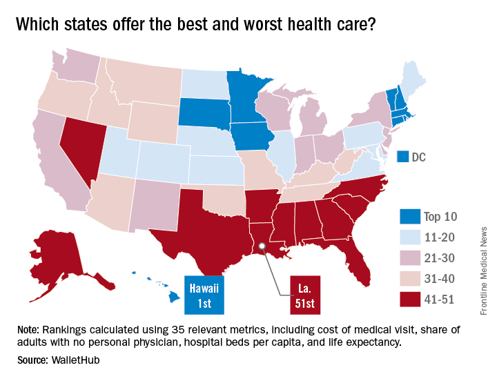
A closer look at some of the individual metrics shows that the District of Columbia has the most physicians per capita and Idaho has the fewest, Medicare acceptance is highest among physicians in North Dakota and lowest in Hawaii, and infant mortality is lowest in New Hampshire and highest in Mississippi, according to the WalletHub analysis, which was based on data from 19 sources, including the Centers for Medicare & Medicaid Services, the Association of American Medical Colleges, and the Social Science Research Council.
IV ketamine proves superior to active placebo in low, high doses
MIAMI – Intravenous ketamine in a range of doses is superior to active placebo, according to analyses from a study of the drug for treatment-resistant depression.
Most of the effect was attributable to differences recorded at Day 1 of the 3-day study, according to George I. Papakostas, MD, scientific director of the Massachusetts General Hospital Clinical Trials Network and Institute and coinvestigator of the study, who presented these findings at a meeting of the American Society of Clinical Psychopharmacology, formerly the New Clinical Drug Evaluation meeting.
The 99 adults with treatment-resistant depression – primarily white women in their mid-40s – were randomly assigned either to an active placebo group given 0.045 mg/kg of midazolam or to one of four treatment arms given a single infusion of intravenous ketamine at either 0.1 mg/kg, 0.2 mg/kg, 0.5 mg/kg, or 1.0 mg/kg.
Baseline scores on the 6-item Hamilton Depression Rating Scale (HAMD-6) ranged between 12.6 and 13.1 across the study.
To determine the efficacy of intravenous ketamine at different doses over the course of 72 hours, Dr. Papakostas, who also directs treatment-resistant depression studies at Massachusetts General, and his colleagues used multiple statistical models. The first analysis was a comparison of the effects of the active placebo and all ketamine groups combined at Day 1 and at Day 3.
At Day 1, the change in baseline HAMD-6 scores for all the ketamine arms combined, compared with the active placebo group, was statistically significant (P = .0278). At Day 3, the change in baseline HAMD-6 scores for the combined ketamine groups, compared with the active placebo arm, also was statistically significant (P = .0391).
A secondary analysis of the patient-reported Symptoms of Depression Questionnaire also showed a statistically significant improvement (P = .09) from baseline in the combined ketamine groups, compared with the active placebo group.
At Day 1, the combined ketamine groups’ changes from baseline HAMD-6 were –3.25 with an effect size of 0.86, a statistically significant finding. However, by the Day 3, the combined ketamine groups’ effects size fell away. “There is no longer a statistically significant difference, so it’s a rapid effect – like we’ve seen in the other studies for the combined doses – but it is not an effect that is sustained,” said Dr. Papakostas, also an associate professor of psychiatry at Harvard Medical School, Boston.
For the individual doses, compared with active placebo, the ketamine 0.1 mg/kg arm had an overall –0.35 change in baseline HAMD-6 scores, which Dr. Papakostas said had “a large effect size of 0.82.”
Dr. Papakostas also said the ketamine 0.2 mg/kg arm “did not really seem to move things around at all.” Meanwhile, the 0.5 mg/kg and 1.0 mg/kg arms each had “big differences” in baseline HAMD-6 scores, compared with active placebo, of –4.79 and –3.76, respectively. They also exhibited statistically significant effect sizes of 1.21 and 0.95 at Day 1, respectively. However, at Day 3, there were neither numerical nor statistical differences, indicating the effect is not sustained.
Changes in the Symptoms of Depression Questionnaire for the combined drug arms at Day 1 were statistically significant with an unadjusted P value of .07 and an adjusted P value of .13.
Results for the Clinician Administered Dissociative States Scale showed that neither the ketamine 0.1 mg/kg arm nor the ketamine 0.2 mg/kg arm separated from active placebo, while the ketamine 0.5 mg/kg arm and the ketamine 1.0 mg/kg arm were each different from active placebo to numerically and statistically significant degrees. Each of the 0.5 mg/kg and the 1.0 mg/kg ketamine arms were associated with rises in blood pressure, according to Dr. Papakostas.
“So, it seems as though the doses that caused a dissociation seemed to cause a clinical effect that is equivalent, whereas in the lower doses, there didn’t seem to be any dissociative effects or blood pressure effects,” Dr. Papakostas said. “If you combine the findings, in my opinion, there is a signal in the 0.1 mg/kg treatment arm, even though it just misses it on the P value.”
Dr. Papakostas said that, although more data are needed to determine optimal dosing and a clearer risk-benefit ratio, the results suggested that intravenous ketamine could offer transient, beneficial effects for patients with treatment-resistant depression.
Dr. Papakostas is the scientific director of the MGH Clinical Trials Network and Institute. This study’s coinvestigator, Maurizio Fava, MD, has numerous relevant financial ties to industry. This trial was part of the National Institute of Mental Health’s Rapidly-Acting Treatments for Treatment-Resistant Depression research program.
[email protected]
On Twitter @whitneymcknight
FROM THE ASCP ANNUAL MEETING
Key clinical point:
Major finding: Ketamine’s effect size and improvement from baseline depression scores showed significant separation from placebo in most analyses conducted in this study.
Data source: Multicenter, randomly controlled, double-blind study of 99 adults with treatment-resistant depression given active placebo or various doses of intravenous ketamine.
Disclosures: Dr. Papakostas is the scientific director of the Massachusetts General Hospital Clinical Trials Network and Institute. This study’s coinvestigator, Dr. Maurizio Fava, has numerous relevant financial ties to industry. This trial was part of the National Institute of Mental Health’s Rapidly-Acting Treatments for Treatment-Resistant Depression research program.
VIDEO: How to prevent, manage perinatal HIV infection
PARK CITY, UTAH – Despite notable progress in recent years, . Early recognition and treatment of HIV infection in pregnancy, prophylaxis for at-risk women, and retention of infected women in postpartum HIV care remain important goals, but they aren’t always met.
In a wide-ranging interview at the annual scientific meeting of the Infectious Diseases Society for Obstetrics and Gynecology, Gweneth Lazenby, MD, associate professor of obstetrics and gynecology at the Medical University of South Carolina, Charleston, explained what to do to improve the situation. Among the many pearls she shared: One HIV test isn’t enough for at-risk women.
AT IDSOG

APAP improves aerophagia symptoms
Switching continuous positive airway pressure–treated patients to autotitrating positive airway pressure (APAP) systems resulted in reduced severity of patient-reported aerophagia symptoms, according to results from a double-blind, randomized study.
Aerophagia, the swallowing of air leading to gastrointestinal distress, is a frequently reported adverse effect among people treated for obstructive sleep apnea with continuous positive airway pressure (CPAP).
The APAP-treated group saw significantly reduced median therapeutic pressure levels compared with the CPAP-treated patients (9.8 vs. 14.0 cm H2O, P less than .001) and slight but statistically significant reductions in self-reported symptoms of bloating, flatulence, and belching. No significant difference was seen in compliance with therapy between the two treatment groups in this study, published in the August 2017 issue of Journal of Clinical Sleep Medicine (J Clin Sleep Med. 2017;13[7]:881-8).
For their research, Teresa Shirlaw and her colleagues in the sleep clinic at Princess Alexandra Hospital in Woolloongabba, Queensland, Australia, analyzed results from 56 adult patients with sleep apnea who had been recently treated with CPAP and reported bloating, flatulence, or belching following therapy.
Patients were randomized 1:1 to in-clinic nighttime CPAP or APAP for 2 weeks and blinded to treatment assignment, while investigators recorded therapy usage hours, pressure, leak, and residual apnea-hypopnea index across the study period. Most of the subjects (n = 39) used full face masks, while others used nasal-only systems.
The researchers considered differences in PAP therapy usage of at least 30 minutes per night to be statistically significant. The APAP group used the assigned therapy a mean 7 hours per night, vs. 6.8 for the CPAP group. Daytime sleepiness outcomes were also similar for the two treatment groups.
Ms. Shirlaw and her colleagues described the compliance findings as a surprise, noting that an earlier meta-analysis had shown slight improvements in compliance associated with APAP (Syst Rev. 2012;1[1]:20). In clinical practice, patients complaining of aerophagia associated with CPAP are frequently switched to APAP based on the belief that doing so “will lead to improved therapy acceptance and … improved compliance,” they wrote.
The investigators described the self-reporting of aerophagia symptoms as one of the study’s limitations. They surmised that the lack of difference seen for compliance measures might be explained in part by the 30-minute usage increments in the study design (compared with 10-minute increments used in some other studies), and the fact that the cohort had relatively high compliance with CPAP at baseline (5.5 hours/night), suggesting a motivated patient population at entry.
The study received some funding from the government of Queensland, and the authors disclosed no conflicts of interest related to their findings.
FROM THE JOURNAL OF CLINICAL SLEEP MEDICINE
Key clinical point: Sleep apnea patients complaining of aerophagia associated with continuous positive airway pressure may find relief using autotitrating positive airway pressure.
Major finding: The APAP-treated group saw significantly reduced median therapeutic pressure levels compared with the CPAP-treated patients (9.8 vs. 14.0 cm H2O, P less than .001) and slight but statistically significant reductions in self-reported symptoms of bloating, flatulence, and belching.
Data source: A randomized, double-blinded trial of 56 adult sleep apnea patients, with previous CPAP and aerophagia, treated at a hospital sleep clinic in Australia.
Disclosures: The government of Queensland helped fund the study. The authors disclosed no conflicts of interest.
Treating women with opioid use disorders poses unique challenges
The opioid epidemic in the United States is reaching a boiling point, with President Trump calling it a “national emergency” and instructing his administration to use all appropriate authority to respond. Experts say that women are disproportionately affected and require unique treatment approaches.
The rate of prescription opioid–related overdoses increased by 471% among women in 2015, compared with an increase of 218% among men. Heroin deaths among women have risen at more than twice the rate among men, according to a report from the Office of Women’s Health (OWH), part of the U.S. Department of Health & Human Services.
The OWH report, released in July, paints a different picture of addiction for women than for men. Women are more likely to experience chronic pain and turn to prescription opioids for longer periods of time and in higher doses. But women also become dependent at smaller doses and in a shorter period of time. Add to this the fact that psychological and emotional distress are risk factors for opioid abuse among women, but not among men, according to the report.
ACOG guidance
In August, the American College of Obstetricians and Gynecologists (ACOG) updated its recommendations for treatments and best practices related to opioid use among pregnant women (Obstet Gynecol. 2017;130:e81-94).
The committee opinion, developed with the American Society of Addiction Medicine, focuses on tearing down stereotypes about women with substance use disorders that could cause patients to slip through the cracks. ACOG recommended universal screening as a part of regular obstetric care, starting with the first prenatal visit.
While screening can involve laboratory testing, the recommendations focus more on creating a comfortable environment for pregnant women to share substance use history and to have a frank conversation about what treatment options are available.
“The document highlights the use of a verbal screening tool which enables the obstetric provider to have a direct conversation with the patient about their answers,” Maria Mascola, MD, an ob.gyn. at the Marshfield (Wis.) Clinic and lead author of the ACOG committee opinion, said in an interview. “It talks about substance use and then provides an opportunity to understand what substances and how much, why these substances might be bad, why this behavior should be changed, and how obstetricians can try to help the person make those changes.”
ACOG continues to recommend medication-assisted treatment (MAT) – typically with methadone or buprenorphine – as the most effective pathway for pregnant women to deal with substance use disorders. However, in cases in which the patient does not accept treatment with an opioid agonist or the treatment is unavailable, medically supervised withdrawal can be considered. ACOG cautions that relapse rates are high (from 59% to more than 90%) and that withdrawal often involves inpatient care and intensive outpatient follow-up. But recent evidence suggests medically supervised withdrawal is not associated with fetal death or preterm delivery.
“There have been some studies looking at smaller groups that have shown pregnant women going through medically supervised withdrawals and there have been some data from those studies that indicate women may be able to successfully go through this withdrawal without harm to the baby,” Dr. Mascola said. “The information we have on medically supervised withdrawal is a small amount of data, and we definitely need more before this is a primary approach.”
Access to care
Regardless of the treatment approach, the larger issue may be accessibility of care. Just 20% of adults with an opioid use disorder get the treatment and care they need each year, according to the OWH, with access and cost cited as the primary barriers to care. This problem is likely worse in rural areas.
“Rural health care is tougher. There is less access; that is an absolute truth, and it’s a burden then for those women to travel long distances to get the care they need,” Dr. Mascola said. “I think ob.gyns. should advocate for more attention in those areas where patients are underserved.”
One potential solution is for ob.gyns. to become certified in providing buprenorphine, which would allow physicians in rural areas to dispense these approved pharmacotherapies to patients who would otherwise be unable to have the proper treatment and follow-up necessary to prevent relapse, Dr. Mascola said.
There is already some federal funding available for this approach. In 2016, the Health Resources and Services Administration awarded $94 million to health centers across the country to expand substance use services, specifically increasing screening for substance use disorders, improving access to medication-assisted treatment, and training clinicians. Similarly, the Substance Abuse and Mental Health Services Administration recently announced it will allocate an additional $485 million to states through the State Targeted Response to the Opioid Crisis Grants to fund medication-assisted treatment and other services.
Unique challenges
Treating women with opioid use disorder isn’t just about identifying the best treatment approach. Social factors appear to play a larger role among women.

“Another difference with women over men is the prevalence of sexual trauma, as well as being in unhealthy relationships where the women are more likely to be enticed into leaving treatment,” she added.
Trauma among women with substance abuse disorders is prevalent, with 55%-99% of women reporting experiencing some form of trauma, compared with 36%-51% of the general population, according to the OWH report.
Beyond exploratory research, there needs to be a major shift in the public perception of opioid substance use, which currently does not approach the disorder as a chronic disease, according to Dr. Jones.
“The treatment process cannot just involve a detoxification program and then send patients off because that will commonly just end in relapse.” Dr. Jones said. “We need to approach substance use disorders with a recovery-oriented system of care in order to create a true safety net they can rely on.”
[email protected]
On Twitter @eaztweets
The opioid epidemic in the United States is reaching a boiling point, with President Trump calling it a “national emergency” and instructing his administration to use all appropriate authority to respond. Experts say that women are disproportionately affected and require unique treatment approaches.
The rate of prescription opioid–related overdoses increased by 471% among women in 2015, compared with an increase of 218% among men. Heroin deaths among women have risen at more than twice the rate among men, according to a report from the Office of Women’s Health (OWH), part of the U.S. Department of Health & Human Services.
The OWH report, released in July, paints a different picture of addiction for women than for men. Women are more likely to experience chronic pain and turn to prescription opioids for longer periods of time and in higher doses. But women also become dependent at smaller doses and in a shorter period of time. Add to this the fact that psychological and emotional distress are risk factors for opioid abuse among women, but not among men, according to the report.
ACOG guidance
In August, the American College of Obstetricians and Gynecologists (ACOG) updated its recommendations for treatments and best practices related to opioid use among pregnant women (Obstet Gynecol. 2017;130:e81-94).
The committee opinion, developed with the American Society of Addiction Medicine, focuses on tearing down stereotypes about women with substance use disorders that could cause patients to slip through the cracks. ACOG recommended universal screening as a part of regular obstetric care, starting with the first prenatal visit.
While screening can involve laboratory testing, the recommendations focus more on creating a comfortable environment for pregnant women to share substance use history and to have a frank conversation about what treatment options are available.
“The document highlights the use of a verbal screening tool which enables the obstetric provider to have a direct conversation with the patient about their answers,” Maria Mascola, MD, an ob.gyn. at the Marshfield (Wis.) Clinic and lead author of the ACOG committee opinion, said in an interview. “It talks about substance use and then provides an opportunity to understand what substances and how much, why these substances might be bad, why this behavior should be changed, and how obstetricians can try to help the person make those changes.”
ACOG continues to recommend medication-assisted treatment (MAT) – typically with methadone or buprenorphine – as the most effective pathway for pregnant women to deal with substance use disorders. However, in cases in which the patient does not accept treatment with an opioid agonist or the treatment is unavailable, medically supervised withdrawal can be considered. ACOG cautions that relapse rates are high (from 59% to more than 90%) and that withdrawal often involves inpatient care and intensive outpatient follow-up. But recent evidence suggests medically supervised withdrawal is not associated with fetal death or preterm delivery.
“There have been some studies looking at smaller groups that have shown pregnant women going through medically supervised withdrawals and there have been some data from those studies that indicate women may be able to successfully go through this withdrawal without harm to the baby,” Dr. Mascola said. “The information we have on medically supervised withdrawal is a small amount of data, and we definitely need more before this is a primary approach.”
Access to care
Regardless of the treatment approach, the larger issue may be accessibility of care. Just 20% of adults with an opioid use disorder get the treatment and care they need each year, according to the OWH, with access and cost cited as the primary barriers to care. This problem is likely worse in rural areas.
“Rural health care is tougher. There is less access; that is an absolute truth, and it’s a burden then for those women to travel long distances to get the care they need,” Dr. Mascola said. “I think ob.gyns. should advocate for more attention in those areas where patients are underserved.”
One potential solution is for ob.gyns. to become certified in providing buprenorphine, which would allow physicians in rural areas to dispense these approved pharmacotherapies to patients who would otherwise be unable to have the proper treatment and follow-up necessary to prevent relapse, Dr. Mascola said.
There is already some federal funding available for this approach. In 2016, the Health Resources and Services Administration awarded $94 million to health centers across the country to expand substance use services, specifically increasing screening for substance use disorders, improving access to medication-assisted treatment, and training clinicians. Similarly, the Substance Abuse and Mental Health Services Administration recently announced it will allocate an additional $485 million to states through the State Targeted Response to the Opioid Crisis Grants to fund medication-assisted treatment and other services.
Unique challenges
Treating women with opioid use disorder isn’t just about identifying the best treatment approach. Social factors appear to play a larger role among women.
“Another difference with women over men is the prevalence of sexual trauma, as well as being in unhealthy relationships where the women are more likely to be enticed into leaving treatment,” she added.
Trauma among women with substance abuse disorders is prevalent, with 55%-99% of women reporting experiencing some form of trauma, compared with 36%-51% of the general population, according to the OWH report.
Beyond exploratory research, there needs to be a major shift in the public perception of opioid substance use, which currently does not approach the disorder as a chronic disease, according to Dr. Jones.
“The treatment process cannot just involve a detoxification program and then send patients off because that will commonly just end in relapse.” Dr. Jones said. “We need to approach substance use disorders with a recovery-oriented system of care in order to create a true safety net they can rely on.”
[email protected]
On Twitter @eaztweets
How to manage submassive pulmonary embolism
The case
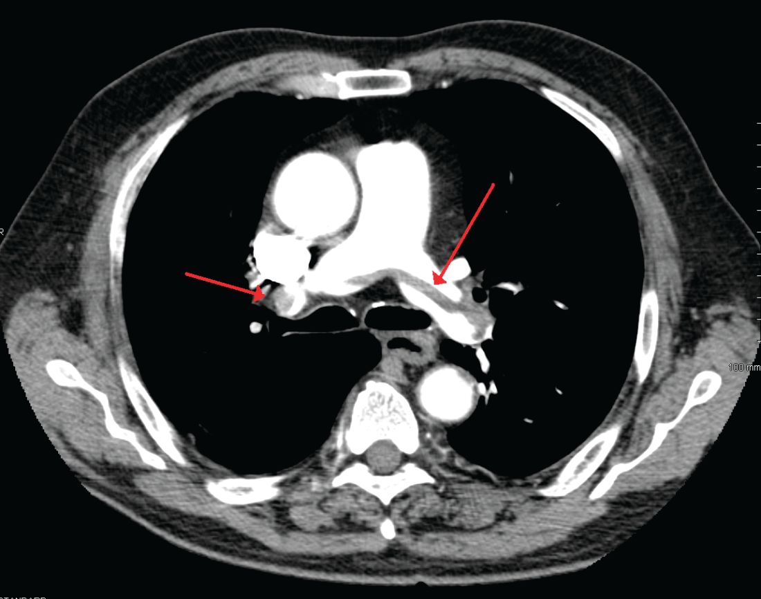
A 49-year-old morbidly obese woman presented to the emergency department with shortness of breath and abdominal distention. On presentation, her blood pressure was 100/60 mm Hg with a heart rate of 110, respiratory rate of 24, and a pulse oximetric saturation (SpO2) of 86% on room air. Troponin T was elevated at 0.3 ng/mL. Computed tomography (CT) of the chest with intravenous contrast showed saddle pulmonary embolism (PE) with dilated right ventricle (RV). CT abdomen/pelvis revealed a very large uterine mass with diffuse lymphadenopathy.
Heparin infusion was started promptly. Echocardiogram demonstrated RV strain. Findings on duplex ultrasound of the lower extremities were consistent with acute deep vein thromboses (DVT) involving the left common femoral vein and the right popliteal vein. Biopsy of a supraclavicular lymph node showed high grade undifferentiated carcinoma most likely of uterine origin.
Clinical questions
What, if any, therapeutic options should be considered beyond standard systemic anticoagulation? Is there a role for:
1. Systemic thrombolysis?
2. Catheter-directed thrombolysis (CDT)?
3. Inferior vena cava (IVC) filter placement?
What is the appropriate management of “submassive” PE?
In the case of massive PE, where the thrombus is located in the central pulmonary vasculature and associated with hypotension due to impaired cardiac output, systemic thrombolysis, embolectomy, and CDT are indicated as potentially life-saving measures. However, the evidence is less clear when the PE is large and has led to RV strain, but without overt hemodynamic instability. This is commonly known as an intermediate risk or “submassive” PE. Submassive PE based on American Heart Association (AHA) guidelines is:1
An acute PE without systemic hypotension (systolic blood pressure less than 90 mm Hg) but with either RV dysfunction or myocardial necrosis. RV dysfunction is defined by the presence of at least one of these following:
• RV dilation (apical 4-chamber RV diameter divided by LV diameter greater than 0.9) or RV systolic dysfunction on echocardiography;
• RV dilation on CT, elevation of BNP (greater than 90 pg/mL), elevation of N-terminal pro-BNP (greater than 500 pg/mL);
• Electrocardiographic changes (new complete or incomplete right bundle branch block, anteroseptal ST elevation or depression, or anteroseptal T-wave inversion).
Myocardial necrosis is defined as elevated troponin I (greater than 0.4 ng/mL) or elevated troponin T (greater than 0.1 ng/mL).
Why is submassive PE of clinical significance?
In 1999, analysis of the International Cooperative Pulmonary Embolism Registry (ICOPER) revealed that RV dysfunction in PE patients was associated with a near doubling of the 3-month mortality risk (hazard ratio 2.0, 1.3-2.9).2 Given this increased risk, one could draw the logical conclusion that we need to treat submassive PE more aggressively than PE without RV strain. But will this necessarily result in a better outcome for the patient given the 3% risk of intracranial hemorrhage associated with thrombolytic therapy?
In the clinical scenario above, the patient did meet the definition of submassive PE. While the patient did not experience systemic hypotension, she did have RV dilation on CT, RV systolic dysfunction on echo as well as an elevated Troponin T level. In addition to starting anticoagulant therapy, what more should be done to increase her probability of a good outcome?
The AHA recommends that systemic thrombolysis and CDT be considered for patients with acute submassive PE if they have clinical evidence of adverse prognosis, including worsening respiratory failure, severe RV dysfunction, or major myocardial necrosis and low risk of bleeding complications (Class IIB; Level of Evidence C).1
The 2016 American College of Chest Physicians (CHEST) guidelines update3 recommends systemically administered thrombolytic therapy over no therapy in selected patients with acute PE who deteriorate after starting anticoagulant therapy but have yet to develop hypotension and who have a low bleeding risk (Grade 2C recommendation).
Systemic thrombolysis
Systemic thrombolysis is administered as an intravenous thrombolytic infusion delivered over a period of time. The Food and Drug Administration–approved thrombolytic drugs currently include tissue plasminogen activator (tPA)/alteplase, streptokinase and urokinase.
Efficacy of low dose thrombolysis was studied in MOPETT 2013,5 a single-center, prospective, randomized, open label study, in which 126 participants found to have submassive PE based on symptoms and CT angiographic or ventilation/perfusion scan data received either 50 mg tPA plus heparin or heparin anticoagulation alone. The composite endpoint of pulmonary hypertension and recurrent PE at 28 months was 16% in the tPA group compared to 63% in the control group (P less than .001). Systemic thrombolysis was associated with lower risk of pulmonary hypertension and recurrent PE, although no mortality benefit was seen in this small study.
In the randomized, double-blind PEITHO trial (n = 1,006) of 20146 comparing tenecteplase plus heparin versus heparin in the submassive PE patients, the primary outcomes of death and hemodynamic decompensation occurred in 2.6% of the tenecteplase group, compared to 5.6% in the placebo group (P = .02). Thrombolytic therapy was associated with 2% rate of hemorrhagic stroke, whereas hemorrhagic stroke in the placebo group was 0.2% (P = .03). In this case, systemic thrombolysis was associated with a 3% lower risk of death and hemodynamic instability, but also a 1.8% increased risk of hemorrhagic stroke.
Catheter-directed thrombolysis (CDT)
CDT was originally developed to treat arterial, dialysis graft and deep vein thromboses, but is now approved by the FDA for the treatment of acute submassive or massive PE.
A wire is passed through the embolus and a multihole infusion catheter is placed, through which a thrombolytic drug is infused over 12-24 hours. The direct delivery of the drug into the thrombus is thought to be as effective as systemic therapy but with a lower risk of bleeding. If more rapid thrombus removal is indicated due to large clot burden and hemodynamic instability, mechanical therapies, such as fragmentation and aspiration, can be used as an adjunct to CDT. However, these mechanical techniques carry the risk of pulmonary artery injury, and therefore should only be used as a last resort. An ultrasound-emitting wire can be added to the multihole infusion catheter to expedite thrombolysis by ultrasonically disrupting the thrombus, a technique known as ultrasound-enhanced thrombolysis (EKOS).7,10
The ULTIMA 2014 trial,8 a small, randomized, open-label study of Ultrasound-Assisted Catheter Directed Thrombolysis (USAT, the term can be used interchangeably with EKOS) versus heparin anticoagulation alone in 59 patients, was designed to study if the former strategy was better at improving the primary outcome measure of RV/LV ratio in submassive PE patients. The mean reduction in RV/LV ratio was 0.30 +/– 0.20 in the USAT group compared to 0.03 +/– 0.16 in the heparin group (P less than .001). However, no significant difference in mortality or bleeding was observed in the groups at 90-day follow up.
The PERFECT 2015 Trial,9 a multicenter registry-based study, prospectively enrolled 101 patients who received CDT as first-line therapy for massive and submassive PE. Among patients with submassive PE, 97.3% were found to have “clinical success” with this treatment, defined as stabilization of hemodynamics, improvement in pulmonary hypertension and right heart strain, and survival to hospital discharge. There was no major bleeding or intracranial hemorrhage. Subgroup analyses in this study comparing USAT against standard CDT did not reveal significant difference in average pulmonary pressure changes, average thrombolytic doses, or average infusion times.
A prospective single-arm multicenter trial, SEATTLE II 2015,10 evaluated the efficacy of EKOS in a sample of 159 patients. Patients with both massive and submassive PE received approximately 24 mg tPA infused via a catheter over 12-24 hours. The primary efficacy outcome was the chest CT-measured RV/LV ratio decrease from the baseline compared to 48 hours post procedure. The pre- and postprocedure ratio was 1.55 versus 1.13 respectively (P less than .001), indicating that EKOS decreased RV dilation. No intracranial hemorrhage was observed and the investigators did not comment on long-term outcomes such as mortality or quality of life. The study was limited by the lack of a comparison group, such as anticoagulation with heparin as monotherapy, or systemic thrombolysis or standard CDT.
Treatment of submassive PE varies between different institutions. There simply are not adequate data comparing low dose systemic thrombolysis, CDT, EKOS, and standard heparin anticoagulation to make firm recommendations. Some investigators feel low-dose systemic thrombolysis is probably as good as the expensive catheter-based thrombolytic therapies.11,12 Low-dose thrombolytic therapy can be followed by use of oral direct factor Xa inhibitors for maintenance of antithrombotic activity.13
Bottom line
In our institution, the interventional radiology team screens patients who meet criteria for submassive PE on a case-by-case basis. We use pulmonary angiographic data (nature and extent of the thrombus), clinical stability, and analysis of other comorbid conditions to decide the best treatment modality for an individual patient. Our team prefers EKOS for submassive PE patients as well as for massive PE patients and as a rescue procedure for patients who have failed systemic thrombolysis.
Until more data are available to support firm guidelines, we feel establishing multidisciplinary teams composed of interventional radiologists, intensivists, cardiologists, and vascular surgeons is prudent to make individualized decisions and to achieve the best outcomes for our patients.14
IVC filter
Since the patient in this case already has a submassive PE, can she tolerate additional clot burden should her remaining DVT embolize again? Is there a role for IVC filter?
The implantation of IVC filters has increased significantly in the past 30 years, without quality evidence justifying their use.15
The 2016 Antithrombotic Therapy for VTE Disease: CHEST Guideline and Expert Panel Report states clearly: In patients with acute DVT of the leg or PE who are treated with anticoagulants, the use of an IVC filter is not recommended (Grade 1B).3 This recommendation is based on findings of the Prevention du Risque d’Embolie Pulmonaire par Interruption Cave (PREPIC) randomized trial,16 and the recently published PREPIC 2 randomized trial,17 both showing that in anticoagulated patients with PE and DVT, concurrent placement of an IVC filter for 3 months did not reduce recurrent PE, including fatal PE.
CHEST guidelines state that an IVC filter should not be routinely placed as an adjunct in patients with PE and DVT. However, what about in the subgroup of patients with submassive or massive PE in whom another PE would be catastrophic? Clinical data are lacking in this area.
Deshpande et al. reported on a series of six patients with massive PE and cardiopulmonary instability; patients all received an IVC filter with anticoagulation. The short-term outcome was excellent, but long-term follow-up was not done.18 Kucher and colleagues reported that from the ICOPER in 2006, out of the 108 massive PE patients with systolic arterial pressure under 90 mm Hg, 11 patients received adjunctive IVC filter placement. None of these 11 patients developed recurrent PE in 90 days and 10 of them survived at least 90 days; IVC filter placement was associated with a reduction in 90-day mortality. In this study, the placement of an IVC filter was entirely decided by the physicians at different sites.19 In a 2012 study examining case fatality rates in 3,770 patients with acute PE who received pulmonary embolectomy, the data showed that in both unstable and stable patients, case fatality rates were lower in those who received an IVC filter.20
Although the above data are favorable for adjunctive IVC filter placement in massive PE patients, at least in short-term outcomes, the small size and lack of randomization preclude establishment of evidence-based guidelines. The 2016 CHEST guidelines point out that as it is uncertain if there is benefit to place an IVC filter adjunctively in anticoagulated patients with severe PE, in this specific subgroup of patients, the recommendation against insertion of an IVC filter in patients with acute PE who are anticoagulated may not apply.3
Bottom line
There is no evidence-based guideline as to whether IVC filters should be placed adjunctively in patients with submassive or massive PE; however, based on expert consensus, it may be appropriate to place an IVC filter as an adjunct to anticoagulation in patients with severe PE. The decision should be individualized based on each patient’s characteristics, preferences, and institutional expertise.
In our case, in hope of preventing further embolic burden, the patient received an IVC filter the day after presentation. Despite the initiation of anticoagulation with heparin, she remained tachycardic and tachypneic, prompting referral for CDT. The interventional radiology team did not feel that she was a good candidate, given her persistent vaginal bleeding and widely metastatic uterine carcinoma. She was switched to therapeutic enoxaparin after no further invasive intervention was deemed appropriate. Her respiratory status did not improve and bilevel positive airway pressure was initiated. Taking into consideration the terminal nature of her cancer, she ultimately elected to pursue comfort care and died shortly afterward.
Acknowledgements
The authors would like to thank Benjamin A. Hohmuth, MD, A. Joseph Layon, MD, and Luis L. Nadal, MD, for their review of the article and invaluable feedback.
Dr. Wenqian Wang, Dr. Vedamurthy, and Dr. Wang are based in the department of hospital medicine at The Medicine Institute, Geisinger Health System, Danville, Penn. Contact Dr. Wenqian Wang at [email protected].
Key Points
• Use pulmonary angiographic data, clinical stability, and analysis of other comorbid conditions to decide the best treatment modality.
• Our team prefers ultrasound-enhanced thrombolysis (EKOS) for submassive PE patients, massive PE patients, and as a rescue procedure for patients who fail systemic thrombolysis.
• Establishing multidisciplinary teams composed of interventional radiologists, intensivists, cardiologists, and vascular surgeons is prudent to make individualized decisions.
• It may be appropriate to place an IVC filter as an adjunct to anticoagulation in patients with severe PE.
References
1. Jaff MR, McMurtry MS, Archer SL, et al. Management of massive and submassive pulmonary embolism, iliofemoral deep vein thrombosis, and chronic thromboembolic pulmonary hypertension: a scientific statement from the American Heart Association. Circulation. 2011;123:1788-1830.
2. Goldhaber SZ, Visani L, De Rosa M. Acute pulmonary embolism: clinical outcomes in the International Cooperative Pulmonary Embolism Registry (ICOPER). Lancet. 1999;353:1386-9.
3. Kearon C, Akl EA, Ornelas J, et al. Antithrombotic Therapy for VTE Disease: CHEST Guideline and Expert Panel Report. Chest. 2016;149:315-52.
4. Konstantinides S, Geibel A, Heusel G, Heinrich F, Kasper W. Management Strategies and Prognosis of Pulmonary Embolism-3 Trial Investigators. Heparin plus alteplase compared with heparin alone in patients with submassive pulmonary embolism. N Engl J Med. 2002;347:1143-50.
5. Sharifi M, Bay C, Skrocki L, Rahimi F, Mehdipour M, “MOPETT” Investigators. Moderate pulmonary embolism treated with thrombolysis (from the “MOPETT” Trial). Am J Cardiol. 2013;111:273-7.
6. Meyer G, Vicaut E, Danays T, et al. Fibrinolysis for patients with intermediate-risk pulmonary embolism. N Engl J Med. 2014;370:1402-11.
7. Kuo WT. Endovascular therapy for acute pulmonary embolism. J Vasc Interv Radiol 2012;23:167-79. e164
8. Kucher N, Boekstegers P, Muller OJ, et al. Randomized, controlled trial of ultrasound-assisted catheter-directed thrombolysis for acute intermediate-risk pulmonary embolism. Circulation. 2014;129:479-86.
9. Kuo WT, Banerjee A, Kim PS, et al. Pulmonary Embolism Response to Fragmentation, Embolectomy, and Catheter Thrombolysis (PERFECT): Initial Results From a Prospective Multicenter Registry. Chest. 2015;148:667-73.
10. Piazza G, Hohlfelder B, Jaff MR, et al. A Prospective, Single-Arm, Multicenter Trial of Ultrasound-Facilitated, Catheter-Directed, Low-Dose Fibrinolysis for Acute Massive and Submassive Pulmonary Embolism: The SEATTLE II Study. JACC Cardiovasc Interv. 2015;8:1382-92.
11. Sharifi M. Systemic Full Dose, Half Dose, and Catheter Directed Thrombolysis for Pulmonary Embolism. When to Use and How to Choose? Curr Treat Options Cardiovasc Med. 2016;18:31.
12. Wang C, Zhai Z, Yang Y, et al. Efficacy and safety of low dose recombinant tissue-type plasminogen activator for the treatment of acute pulmonary thromboembolism: a randomized, multicenter, controlled trial. Chest. 2010;137:254-62.
13. Sharifi M, Vajo Z, Freeman W, Bay C, Sharifi M, Schwartz F. Transforming and simplifying the treatment of pulmonary embolism: “safe dose” thrombolysis plus new oral anticoagulants. Lung. 2015;193:369-74.
14. Kabrhel C, Rosovsky R, Channick R, et al. A Multidisciplinary Pulmonary Embolism Response Team: Initial 30-Month Experience With a Novel Approach to Delivery of Care to Patients With Submassive and Massive Pulmonary Embolism. Chest. 2016;150:384-93.
15. Lessne ML, Sing RF. Counterpoint: Do the Benefits Outweigh the Risks for Most Patients Under Consideration for inferior vena cava filters? No. Chest. 2016; 150(6):1182-4.
16. The PREPIC Study Group. Eight-year follow-up of patients with permanent vena cava filters in the prevention of pulmonary embolism: the PREPIC (Prevention du Risque d’Embolie Pulmonaire par Interruption Cave) randomized study. Circulation. 2005;112(3):416-22.
17. Mismetti P, Laporte S, Pellerin O, et al. Effect of a retrievable inferior vena cava filter plus anticoagulation vs. anticoagulation alone on risk of recurrent pulmonary embolism: a randomized clinical trial. JAMA. 2015. 313(16):1627-35.
18. Deshpande KS, Hatem C, Karwa M, et al. The use of inferior vena cava filter as a treatment modality for massive pulmonary embolism. A case series and review of pathophysiology. Respir Med. 2002.96(12):984-9.
19. Kucher N, Rossi E, De Rosa M, et al. Massive Pulmonary embolism. Circulation. 2006;113(4):577-82.
20. Stein P, Matta F. Case Fatality Rate with Pulmonary Embolectomy for Acute Pulmonary Embolism. Am J Med. 2012;125:471-7.
The case
A 49-year-old morbidly obese woman presented to the emergency department with shortness of breath and abdominal distention. On presentation, her blood pressure was 100/60 mm Hg with a heart rate of 110, respiratory rate of 24, and a pulse oximetric saturation (SpO2) of 86% on room air. Troponin T was elevated at 0.3 ng/mL. Computed tomography (CT) of the chest with intravenous contrast showed saddle pulmonary embolism (PE) with dilated right ventricle (RV). CT abdomen/pelvis revealed a very large uterine mass with diffuse lymphadenopathy.
Heparin infusion was started promptly. Echocardiogram demonstrated RV strain. Findings on duplex ultrasound of the lower extremities were consistent with acute deep vein thromboses (DVT) involving the left common femoral vein and the right popliteal vein. Biopsy of a supraclavicular lymph node showed high grade undifferentiated carcinoma most likely of uterine origin.
Clinical questions
What, if any, therapeutic options should be considered beyond standard systemic anticoagulation? Is there a role for:
1. Systemic thrombolysis?
2. Catheter-directed thrombolysis (CDT)?
3. Inferior vena cava (IVC) filter placement?
What is the appropriate management of “submassive” PE?
In the case of massive PE, where the thrombus is located in the central pulmonary vasculature and associated with hypotension due to impaired cardiac output, systemic thrombolysis, embolectomy, and CDT are indicated as potentially life-saving measures. However, the evidence is less clear when the PE is large and has led to RV strain, but without overt hemodynamic instability. This is commonly known as an intermediate risk or “submassive” PE. Submassive PE based on American Heart Association (AHA) guidelines is:1
An acute PE without systemic hypotension (systolic blood pressure less than 90 mm Hg) but with either RV dysfunction or myocardial necrosis. RV dysfunction is defined by the presence of at least one of these following:
• RV dilation (apical 4-chamber RV diameter divided by LV diameter greater than 0.9) or RV systolic dysfunction on echocardiography;
• RV dilation on CT, elevation of BNP (greater than 90 pg/mL), elevation of N-terminal pro-BNP (greater than 500 pg/mL);
• Electrocardiographic changes (new complete or incomplete right bundle branch block, anteroseptal ST elevation or depression, or anteroseptal T-wave inversion).
Myocardial necrosis is defined as elevated troponin I (greater than 0.4 ng/mL) or elevated troponin T (greater than 0.1 ng/mL).
Why is submassive PE of clinical significance?
In 1999, analysis of the International Cooperative Pulmonary Embolism Registry (ICOPER) revealed that RV dysfunction in PE patients was associated with a near doubling of the 3-month mortality risk (hazard ratio 2.0, 1.3-2.9).2 Given this increased risk, one could draw the logical conclusion that we need to treat submassive PE more aggressively than PE without RV strain. But will this necessarily result in a better outcome for the patient given the 3% risk of intracranial hemorrhage associated with thrombolytic therapy?
In the clinical scenario above, the patient did meet the definition of submassive PE. While the patient did not experience systemic hypotension, she did have RV dilation on CT, RV systolic dysfunction on echo as well as an elevated Troponin T level. In addition to starting anticoagulant therapy, what more should be done to increase her probability of a good outcome?
The AHA recommends that systemic thrombolysis and CDT be considered for patients with acute submassive PE if they have clinical evidence of adverse prognosis, including worsening respiratory failure, severe RV dysfunction, or major myocardial necrosis and low risk of bleeding complications (Class IIB; Level of Evidence C).1
The 2016 American College of Chest Physicians (CHEST) guidelines update3 recommends systemically administered thrombolytic therapy over no therapy in selected patients with acute PE who deteriorate after starting anticoagulant therapy but have yet to develop hypotension and who have a low bleeding risk (Grade 2C recommendation).
Systemic thrombolysis
Systemic thrombolysis is administered as an intravenous thrombolytic infusion delivered over a period of time. The Food and Drug Administration–approved thrombolytic drugs currently include tissue plasminogen activator (tPA)/alteplase, streptokinase and urokinase.
Efficacy of low dose thrombolysis was studied in MOPETT 2013,5 a single-center, prospective, randomized, open label study, in which 126 participants found to have submassive PE based on symptoms and CT angiographic or ventilation/perfusion scan data received either 50 mg tPA plus heparin or heparin anticoagulation alone. The composite endpoint of pulmonary hypertension and recurrent PE at 28 months was 16% in the tPA group compared to 63% in the control group (P less than .001). Systemic thrombolysis was associated with lower risk of pulmonary hypertension and recurrent PE, although no mortality benefit was seen in this small study.
In the randomized, double-blind PEITHO trial (n = 1,006) of 20146 comparing tenecteplase plus heparin versus heparin in the submassive PE patients, the primary outcomes of death and hemodynamic decompensation occurred in 2.6% of the tenecteplase group, compared to 5.6% in the placebo group (P = .02). Thrombolytic therapy was associated with 2% rate of hemorrhagic stroke, whereas hemorrhagic stroke in the placebo group was 0.2% (P = .03). In this case, systemic thrombolysis was associated with a 3% lower risk of death and hemodynamic instability, but also a 1.8% increased risk of hemorrhagic stroke.
Catheter-directed thrombolysis (CDT)
CDT was originally developed to treat arterial, dialysis graft and deep vein thromboses, but is now approved by the FDA for the treatment of acute submassive or massive PE.
A wire is passed through the embolus and a multihole infusion catheter is placed, through which a thrombolytic drug is infused over 12-24 hours. The direct delivery of the drug into the thrombus is thought to be as effective as systemic therapy but with a lower risk of bleeding. If more rapid thrombus removal is indicated due to large clot burden and hemodynamic instability, mechanical therapies, such as fragmentation and aspiration, can be used as an adjunct to CDT. However, these mechanical techniques carry the risk of pulmonary artery injury, and therefore should only be used as a last resort. An ultrasound-emitting wire can be added to the multihole infusion catheter to expedite thrombolysis by ultrasonically disrupting the thrombus, a technique known as ultrasound-enhanced thrombolysis (EKOS).7,10
The ULTIMA 2014 trial,8 a small, randomized, open-label study of Ultrasound-Assisted Catheter Directed Thrombolysis (USAT, the term can be used interchangeably with EKOS) versus heparin anticoagulation alone in 59 patients, was designed to study if the former strategy was better at improving the primary outcome measure of RV/LV ratio in submassive PE patients. The mean reduction in RV/LV ratio was 0.30 +/– 0.20 in the USAT group compared to 0.03 +/– 0.16 in the heparin group (P less than .001). However, no significant difference in mortality or bleeding was observed in the groups at 90-day follow up.
The PERFECT 2015 Trial,9 a multicenter registry-based study, prospectively enrolled 101 patients who received CDT as first-line therapy for massive and submassive PE. Among patients with submassive PE, 97.3% were found to have “clinical success” with this treatment, defined as stabilization of hemodynamics, improvement in pulmonary hypertension and right heart strain, and survival to hospital discharge. There was no major bleeding or intracranial hemorrhage. Subgroup analyses in this study comparing USAT against standard CDT did not reveal significant difference in average pulmonary pressure changes, average thrombolytic doses, or average infusion times.
A prospective single-arm multicenter trial, SEATTLE II 2015,10 evaluated the efficacy of EKOS in a sample of 159 patients. Patients with both massive and submassive PE received approximately 24 mg tPA infused via a catheter over 12-24 hours. The primary efficacy outcome was the chest CT-measured RV/LV ratio decrease from the baseline compared to 48 hours post procedure. The pre- and postprocedure ratio was 1.55 versus 1.13 respectively (P less than .001), indicating that EKOS decreased RV dilation. No intracranial hemorrhage was observed and the investigators did not comment on long-term outcomes such as mortality or quality of life. The study was limited by the lack of a comparison group, such as anticoagulation with heparin as monotherapy, or systemic thrombolysis or standard CDT.
Treatment of submassive PE varies between different institutions. There simply are not adequate data comparing low dose systemic thrombolysis, CDT, EKOS, and standard heparin anticoagulation to make firm recommendations. Some investigators feel low-dose systemic thrombolysis is probably as good as the expensive catheter-based thrombolytic therapies.11,12 Low-dose thrombolytic therapy can be followed by use of oral direct factor Xa inhibitors for maintenance of antithrombotic activity.13
Bottom line
In our institution, the interventional radiology team screens patients who meet criteria for submassive PE on a case-by-case basis. We use pulmonary angiographic data (nature and extent of the thrombus), clinical stability, and analysis of other comorbid conditions to decide the best treatment modality for an individual patient. Our team prefers EKOS for submassive PE patients as well as for massive PE patients and as a rescue procedure for patients who have failed systemic thrombolysis.
Until more data are available to support firm guidelines, we feel establishing multidisciplinary teams composed of interventional radiologists, intensivists, cardiologists, and vascular surgeons is prudent to make individualized decisions and to achieve the best outcomes for our patients.14
IVC filter
Since the patient in this case already has a submassive PE, can she tolerate additional clot burden should her remaining DVT embolize again? Is there a role for IVC filter?
The implantation of IVC filters has increased significantly in the past 30 years, without quality evidence justifying their use.15
The 2016 Antithrombotic Therapy for VTE Disease: CHEST Guideline and Expert Panel Report states clearly: In patients with acute DVT of the leg or PE who are treated with anticoagulants, the use of an IVC filter is not recommended (Grade 1B).3 This recommendation is based on findings of the Prevention du Risque d’Embolie Pulmonaire par Interruption Cave (PREPIC) randomized trial,16 and the recently published PREPIC 2 randomized trial,17 both showing that in anticoagulated patients with PE and DVT, concurrent placement of an IVC filter for 3 months did not reduce recurrent PE, including fatal PE.
CHEST guidelines state that an IVC filter should not be routinely placed as an adjunct in patients with PE and DVT. However, what about in the subgroup of patients with submassive or massive PE in whom another PE would be catastrophic? Clinical data are lacking in this area.
Deshpande et al. reported on a series of six patients with massive PE and cardiopulmonary instability; patients all received an IVC filter with anticoagulation. The short-term outcome was excellent, but long-term follow-up was not done.18 Kucher and colleagues reported that from the ICOPER in 2006, out of the 108 massive PE patients with systolic arterial pressure under 90 mm Hg, 11 patients received adjunctive IVC filter placement. None of these 11 patients developed recurrent PE in 90 days and 10 of them survived at least 90 days; IVC filter placement was associated with a reduction in 90-day mortality. In this study, the placement of an IVC filter was entirely decided by the physicians at different sites.19 In a 2012 study examining case fatality rates in 3,770 patients with acute PE who received pulmonary embolectomy, the data showed that in both unstable and stable patients, case fatality rates were lower in those who received an IVC filter.20
Although the above data are favorable for adjunctive IVC filter placement in massive PE patients, at least in short-term outcomes, the small size and lack of randomization preclude establishment of evidence-based guidelines. The 2016 CHEST guidelines point out that as it is uncertain if there is benefit to place an IVC filter adjunctively in anticoagulated patients with severe PE, in this specific subgroup of patients, the recommendation against insertion of an IVC filter in patients with acute PE who are anticoagulated may not apply.3
Bottom line
There is no evidence-based guideline as to whether IVC filters should be placed adjunctively in patients with submassive or massive PE; however, based on expert consensus, it may be appropriate to place an IVC filter as an adjunct to anticoagulation in patients with severe PE. The decision should be individualized based on each patient’s characteristics, preferences, and institutional expertise.
In our case, in hope of preventing further embolic burden, the patient received an IVC filter the day after presentation. Despite the initiation of anticoagulation with heparin, she remained tachycardic and tachypneic, prompting referral for CDT. The interventional radiology team did not feel that she was a good candidate, given her persistent vaginal bleeding and widely metastatic uterine carcinoma. She was switched to therapeutic enoxaparin after no further invasive intervention was deemed appropriate. Her respiratory status did not improve and bilevel positive airway pressure was initiated. Taking into consideration the terminal nature of her cancer, she ultimately elected to pursue comfort care and died shortly afterward.
Acknowledgements
The authors would like to thank Benjamin A. Hohmuth, MD, A. Joseph Layon, MD, and Luis L. Nadal, MD, for their review of the article and invaluable feedback.
Dr. Wenqian Wang, Dr. Vedamurthy, and Dr. Wang are based in the department of hospital medicine at The Medicine Institute, Geisinger Health System, Danville, Penn. Contact Dr. Wenqian Wang at [email protected].
Key Points
• Use pulmonary angiographic data, clinical stability, and analysis of other comorbid conditions to decide the best treatment modality.
• Our team prefers ultrasound-enhanced thrombolysis (EKOS) for submassive PE patients, massive PE patients, and as a rescue procedure for patients who fail systemic thrombolysis.
• Establishing multidisciplinary teams composed of interventional radiologists, intensivists, cardiologists, and vascular surgeons is prudent to make individualized decisions.
• It may be appropriate to place an IVC filter as an adjunct to anticoagulation in patients with severe PE.
References
1. Jaff MR, McMurtry MS, Archer SL, et al. Management of massive and submassive pulmonary embolism, iliofemoral deep vein thrombosis, and chronic thromboembolic pulmonary hypertension: a scientific statement from the American Heart Association. Circulation. 2011;123:1788-1830.
2. Goldhaber SZ, Visani L, De Rosa M. Acute pulmonary embolism: clinical outcomes in the International Cooperative Pulmonary Embolism Registry (ICOPER). Lancet. 1999;353:1386-9.
3. Kearon C, Akl EA, Ornelas J, et al. Antithrombotic Therapy for VTE Disease: CHEST Guideline and Expert Panel Report. Chest. 2016;149:315-52.
4. Konstantinides S, Geibel A, Heusel G, Heinrich F, Kasper W. Management Strategies and Prognosis of Pulmonary Embolism-3 Trial Investigators. Heparin plus alteplase compared with heparin alone in patients with submassive pulmonary embolism. N Engl J Med. 2002;347:1143-50.
5. Sharifi M, Bay C, Skrocki L, Rahimi F, Mehdipour M, “MOPETT” Investigators. Moderate pulmonary embolism treated with thrombolysis (from the “MOPETT” Trial). Am J Cardiol. 2013;111:273-7.
6. Meyer G, Vicaut E, Danays T, et al. Fibrinolysis for patients with intermediate-risk pulmonary embolism. N Engl J Med. 2014;370:1402-11.
7. Kuo WT. Endovascular therapy for acute pulmonary embolism. J Vasc Interv Radiol 2012;23:167-79. e164
8. Kucher N, Boekstegers P, Muller OJ, et al. Randomized, controlled trial of ultrasound-assisted catheter-directed thrombolysis for acute intermediate-risk pulmonary embolism. Circulation. 2014;129:479-86.
9. Kuo WT, Banerjee A, Kim PS, et al. Pulmonary Embolism Response to Fragmentation, Embolectomy, and Catheter Thrombolysis (PERFECT): Initial Results From a Prospective Multicenter Registry. Chest. 2015;148:667-73.
10. Piazza G, Hohlfelder B, Jaff MR, et al. A Prospective, Single-Arm, Multicenter Trial of Ultrasound-Facilitated, Catheter-Directed, Low-Dose Fibrinolysis for Acute Massive and Submassive Pulmonary Embolism: The SEATTLE II Study. JACC Cardiovasc Interv. 2015;8:1382-92.
11. Sharifi M. Systemic Full Dose, Half Dose, and Catheter Directed Thrombolysis for Pulmonary Embolism. When to Use and How to Choose? Curr Treat Options Cardiovasc Med. 2016;18:31.
12. Wang C, Zhai Z, Yang Y, et al. Efficacy and safety of low dose recombinant tissue-type plasminogen activator for the treatment of acute pulmonary thromboembolism: a randomized, multicenter, controlled trial. Chest. 2010;137:254-62.
13. Sharifi M, Vajo Z, Freeman W, Bay C, Sharifi M, Schwartz F. Transforming and simplifying the treatment of pulmonary embolism: “safe dose” thrombolysis plus new oral anticoagulants. Lung. 2015;193:369-74.
14. Kabrhel C, Rosovsky R, Channick R, et al. A Multidisciplinary Pulmonary Embolism Response Team: Initial 30-Month Experience With a Novel Approach to Delivery of Care to Patients With Submassive and Massive Pulmonary Embolism. Chest. 2016;150:384-93.
15. Lessne ML, Sing RF. Counterpoint: Do the Benefits Outweigh the Risks for Most Patients Under Consideration for inferior vena cava filters? No. Chest. 2016; 150(6):1182-4.
16. The PREPIC Study Group. Eight-year follow-up of patients with permanent vena cava filters in the prevention of pulmonary embolism: the PREPIC (Prevention du Risque d’Embolie Pulmonaire par Interruption Cave) randomized study. Circulation. 2005;112(3):416-22.
17. Mismetti P, Laporte S, Pellerin O, et al. Effect of a retrievable inferior vena cava filter plus anticoagulation vs. anticoagulation alone on risk of recurrent pulmonary embolism: a randomized clinical trial. JAMA. 2015. 313(16):1627-35.
18. Deshpande KS, Hatem C, Karwa M, et al. The use of inferior vena cava filter as a treatment modality for massive pulmonary embolism. A case series and review of pathophysiology. Respir Med. 2002.96(12):984-9.
19. Kucher N, Rossi E, De Rosa M, et al. Massive Pulmonary embolism. Circulation. 2006;113(4):577-82.
20. Stein P, Matta F. Case Fatality Rate with Pulmonary Embolectomy for Acute Pulmonary Embolism. Am J Med. 2012;125:471-7.
Zika linked to a spectrum of neuroinflammatory diseases
New evidence in support of a link between Zika virus infection and an increase in the incidence of neurological syndromes in adults has come from a prospective, observational study that demonstrates the presence of the infection in both serum and cerebrospinal fluid of patients with new-onset acute neuroinflammatory disease.
From Dec. 5, 2015, to May 10, 2016, 40 patients who were hospitalized for Guillain-Barré syndrome (GBS), meningoencephalitis, or transverse myelitis were evaluated for Zika virus. Of those, 35 (88%) tested positive for Zika, indicating that there is a correlation between the Zika outbreak and recorded increases in neurological syndromes in adults, according to Ivan Rocha Ferreira da Silva, MD, PhD, of the neurology department of Universidade Federal Fluminense in Niteroi, Brazil, and his coauthors (JAMA Neurol. 2017 Aug 14. doi: 10.1001/jamaneurol.2017.1703). Dr. da Silva is now with the department of neurology at Rush University Medical Center, Chicago.
Overall, it appears that Zika virus is associated with the trend for the rapid increase in hospital admissions for certain neurological syndromes, Dr. da Silva and his coauthors said. In addition, “we believe that our method of matching CSF and blood serologic findings offers a substantial aid to minimize [costs and] cross-reactivity in countries with a high prevalence of other concurrent flavivirosis.”
The study cohort was enrolled at a tertiary care, academic hospital in Rio de Janeiro. The median age was 44, and 15 were women. The study was limited by selection of neurological syndromes that have previously been associated with other flaviviruses, the short study period, and the use of patients from only one hospital.
Dr. da Silva reported no financial disclosures. One author reported receiving grants from Conselho Nacional de Desenvolvimento e Pesquisa and Fundação de Amparo à Pesquisa do Estado do Rio de Janeiro. Other study authors reported no financial disclosures.
The 2015 Zika outbreaks in the Americas were notable for the recognition that Zika virus could be associated with neurological conditions. It was found that the overall risk of congenital neurologic abnormalities in fetuses and liveborn children of mothers enrolled in the Centers for Disease Control and Prevention’s Zika Pregnancy Registry with definite laboratory evidence of Zika virus infection during pregnancy was approximately 17 times higher than the expected baseline rate in uninfected mothers. It wasn’t until later, however, that GBS became the first non–pregnancy-related neurological syndrome to be associate with Zika in adults.
It is critically important to understand both the spectrum and frequency of Zika virus–induced neurologic diseases. The article by Dr. da Silva and colleagues in this issue of JAMA Neurology represents an initial approach to this problem. During the reporting period, they found that 93% of the patients with GBS (27 of 29), 71% of the patients with encephalitis (5 of 7), 67% of the patients with transverse myelitis (2 of 3), and the single patient with chronic inflammatory demyelinating polyneuropathy showed evidence of recent Zika virus infection, indicating a link between neurological syndromes and Zika.
However, it should be noted that, because of factors including referral bias, a study such as this cannot determine exact frequencies of Zika virus infection among patients with the syndromes examined, but it may serve to help confirm that Zika can be associated with such syndromes.
Kenneth L. Tyler, MD, is the Louise Baum Endowed Professor and Chair of the department of neurology at the University of Colorado at Denver, Aurora. Karen L. Roos, MD, is the John and Nancy Professor of Neurology at the University of Indiana, Indianapolis. They published these comments in an editorial accompanying the da Silva et al. article in JAMA Neurology (2017 Aug 14. doi: 10.1001/jamaneurol.2017.1471). Neither author reported any financial disclosures.
New evidence in support of a link between Zika virus infection and an increase in the incidence of neurological syndromes in adults has come from a prospective, observational study that demonstrates the presence of the infection in both serum and cerebrospinal fluid of patients with new-onset acute neuroinflammatory disease.
From Dec. 5, 2015, to May 10, 2016, 40 patients who were hospitalized for Guillain-Barré syndrome (GBS), meningoencephalitis, or transverse myelitis were evaluated for Zika virus. Of those, 35 (88%) tested positive for Zika, indicating that there is a correlation between the Zika outbreak and recorded increases in neurological syndromes in adults, according to Ivan Rocha Ferreira da Silva, MD, PhD, of the neurology department of Universidade Federal Fluminense in Niteroi, Brazil, and his coauthors (JAMA Neurol. 2017 Aug 14. doi: 10.1001/jamaneurol.2017.1703). Dr. da Silva is now with the department of neurology at Rush University Medical Center, Chicago.
Overall, it appears that Zika virus is associated with the trend for the rapid increase in hospital admissions for certain neurological syndromes, Dr. da Silva and his coauthors said. In addition, “we believe that our method of matching CSF and blood serologic findings offers a substantial aid to minimize [costs and] cross-reactivity in countries with a high prevalence of other concurrent flavivirosis.”
The study cohort was enrolled at a tertiary care, academic hospital in Rio de Janeiro. The median age was 44, and 15 were women. The study was limited by selection of neurological syndromes that have previously been associated with other flaviviruses, the short study period, and the use of patients from only one hospital.
Dr. da Silva reported no financial disclosures. One author reported receiving grants from Conselho Nacional de Desenvolvimento e Pesquisa and Fundação de Amparo à Pesquisa do Estado do Rio de Janeiro. Other study authors reported no financial disclosures.
FROM JAMA NEUROLOGY
Key clinical point: Increases in neurological syndromes in adults are associated with the Zika epidemic.
Major finding: Of 40 patients who were hospitalized for Guillain-Barré syndrome (GBS), meningoencephalitis, or transverse myelitis, 35 tested positive for Zika.
Data source: A prospective, observational cohort study of 40 patients who were admitted to a hospital in Brazil for a number of neurological conditions.
Disclosures: Dr. da Silva reported no financial disclosures. One author reported receiving grants from Conselho Nacional de Desenvolvimento e Pesquisa and Fundação de Amparo à Pesquisa do Estado do Rio de Janeiro. Other study authors reported no financial disclosures.
Miss the MIPS Webinar? View it Online
The SVS Patient Safety Organization and M2S, in conjunction with the SVS, presented a webinar last month on getting started in the Medicare reimbursement program, including the Merit-based Incentive Payment System (MIPS).
For those who couldn't attend, it is posted, along with the presentation slides, on the Vascular Quality Initiative website's home page. View it today to get up to speed on MIPS and MACRA (Medicare Access and CHIP Reauthorization Act of 2015).
Birth Control Pills for Acne: Tips From Julie Harper at the Summer AAD
Acne treatment options now extend beyond antibiotics, and hormonal therapy, particularly birth control pills (BCPs), may provide clearance of acne in women who may not respond to other therapies. "Challenge [yourselves] to learn how to safely use BCPs," said Dr. Julie Harper, Clinical Associate Professor of Dermatology at the University of Alabama in Birmingham, in the presentation, "Use of Hormonal Therapy for Acne," at the Summer Meeting of the American Academy of Dermatology. The use of BCPs for acne has a strength-of-recommendation grade of A (consistent, good-quality patient-oriented evidence).
According to Dr. Harper, all combination BCPs should work for acne, except progestin-only BCPs, which will make acne worse. Currently, there are 4 BCPs approved by the US Food and Drug Administration for acne: norgestimate-ethinyl estradiol (Ortho Tri-Cyclen); norethindrone acetate-ethinyl estradiol (Estrostep Fe); drospirenone-ethinyl estradiol (Yaz); and drospirenone-ethinyl estradiol-levomefolate calcium (Beyaz). Birth control pills are known to carry risks for venous thromboembolism (VTE), stroke, hypertension, and myocardial infarction; however, they are generally well tolerated in acne patients. "The risk of venous thromboembolism in women who take BCPs is doubled or tripled compared to women who do not take these pills. This sounds scary until you put it into context," said Dr. Harper. She explains the risks to patients using the following 3-6-9-12 model: A woman's baseline risk of having a VTE if she is not on a BCP is approximately 3 in 10,000 women in one year. When she takes a BCP, her risk doubles to 6 per 10,000 women in one year. If she takes a BCP that contains drospirenone, her risk is 9 per 10,000 women in one year. If she gets pregnant, her risk is 12 per 10,000 women in one year.
Dermatologists may be apprehensive to prescribe BCPs, but Dr. Harper provided several important tips on managing patient expectations and monitoring patients. Dr. Harper emphasized that BCPs should be used patiently for acne. "It frequently takes at least 3 cycles of BCPs to see a meaningful change in acne reduction," she advised. She recommended obtaining a thorough medical history and blood pressure measurement prior to prescribing BCPs. However, a Papanicolaou test and bimanual pelvic examination are no longer deemed mandatory prior to initiating a BCP, according to the World Health Organization and the American Congress of Obstetricians and Gynecologists. "While these exams may help to detect cervical cancer and other pelvic diseases, BCPs help to prevent unwanted pregnancies and the risks that accompany those pregnancies," said Dr. Harper. "Remember that BCPs reduce the risk of ovarian, uterine and colorectal cancer and also lessen ovarian cysts and pelvic inflammatory disease." Dermatologists also should inform patients that rifampin and griseofulvin, both anti-infectives, will interact with BCPs, lessening their effectiveness.
A March 2017 study published in Cutis (2017;99:195-201) of US dermatologists' knowledge, comfort, and prescribing practices (N=116) revealed that most dermatologists (95.4%) believe BCPs effectively treat acne; however, only 54% reported prescribing them. The American Academy of Dermatology's guidelines of care for the management of acne vulgaris published in February 2016 (J Am Acad Dermatol. 2016;74:945-973) stated that "estrogen-containing combined oral contraceptives are effective and recommended in the treatment of inflammatory acne in females."
Overall, Dr. Harper's take-home message was that dermatologists should not be afraid to prescribe BCPs, even in teenaged girls (following the onset of menarche). "Birth control pills can be used in younger patients but it is not my first line of treatment," said Dr. Harper. "It is recommended that BCPs not be prescribed for acne until 2 years after the young woman has achieved menarche. When considering whether or not to use a BCP in the early teenage years, keep in mind that these are not short-term treatments. If a BCP does help acne, it will likely need to be maintained for many years." When discussing this treatment in front of parents/guardians, consider referring to it as hormonal therapy and use the term birth control pills only initially.
‘Motivational pharmacotherapy’ engages Latino patients with depression
MIAMI – Approaching treatment as a partnership between clinician and patient can help improve adherence in underserved members of racial/ethnic groups with depression, according to an expert.
“There is plenty of evidence that clinicians are less likely to engage minorities in a participatory way,” Roberto Lewis-Fernández, MD, said during a plenary session at a meeting of the American Society of Clinical Psychopharmacology, formerly the New Clinical Drug Evaluation Unit meeting. “They tend to ask fewer questions [of patients]. They tend to engage [patients] less in clinical decision making.”
This can lead to nonadherence or even discontinuation of therapy, said Dr. Lewis-Fernández, director of the New York State (NYS) Center of Excellence for Cultural Competence, as well as the Anxiety Disorders Clinic and the Hispanic Treatment Program at NYS Psychiatric Institute.

One solution for bridging what Dr. Lewis-Fernández calls the “power differential” between therapist and patient, and improving adherence rates, is to use “motivational pharmacotherapy,” a derivative of motivational interviewing, created by Dr. Lewis-Fernández and his colleagues. With motivational pharmacotherapy, patients are viewed as the experts in their challenges when meeting the needs of their treatment plan. The clinician is the expert partner in the technical aspects of care.
In a 12-week, open-trial pilot study for this intervention in 50 first-generation Latino patients diagnosed with major depressive disorder, Dr. Lewis-Fernández and his colleagues found that 20% of patients discontinued treatment, with a mean therapy duration of 74.2 out of 84 days (Psychiatry. 2013 Fall;76[3]:210-22).This was in comparison to reports in the literature of discontinuation rates among Latino patients ranging from 32% to 53%, and to rates between 36% and 46% in previous studies conducted at Dr. Lewis-Fernández’s own clinic, using similar medications and methods.
They also found that responder and remitter rates were 82% and 68%. The average length of the first clinical visit was 36.7 minutes, and 24.3 minutes for subsequent visits, which Dr. Lewis-Fernández said was compatible with community clinics.
Motivational pharmacotherapy relies on the psychotherapy components of motivational interviewing that address the need for behavioral change and for helping patients reduce their ambivalence about taking antidepressants. Those components are combined with manualized pharmacotherapy, said Dr. Lewis-Fernández, professor of clinical psychiatry at Columbia University, New York.
The language and tone of this kind of intervention must be empathetic and nonconfrontational, he said. “You can’t say to people who are ambivalent, ‘No, you’re wrong. Take your medication.’ Instead, [focus on] the discrepancy between the current situation and the desired state. Then medication can serve as the solution.”
This allows the patient to “roll with their resistance,” he said, rather than meet it head on. In turn, this approach emphasizes the patient’s capacity to advocate for himself or herself.
“You can’t do the treatment without the patient,” Dr. Lewis-Fernández said. “It’s essentially psychoeducation.”
Among some of the tips for conducting this intervention cited by Dr. Lewis-Fernández:
- Ask questions to elicit the patients’ cultural understanding about their illness and what troubles them most about their condition.
- Ask patients’ permission to show them the supportive data for the intervention.
- Ask them about their thoughts and feelings in response to learning the data.
- Use their understanding of the pros and cons of the medication to “negotiate” their engagement.
In previous studies, Dr. Lewis-Fernández said, he and his colleagues analyzed the reasons for nonadherence, which he said often were tied to the “chaos of their lives.” However, he said, there were improvements after the patients engaged in this psychoeducation-enriched intervention.
Not blaming minority patients for poor adherence is important, he said, since their ambivalence takes place in the context of having less access to quality care. Among the many obstacles these patients face in getting the care they need, insufficient clinician training in how to engage them should not have to be one of them, Dr. Lewis-Fernández said. “We should be doing something about this as a profession.”
Dr. Lewis-Fernández said he had no relevant disclosures. The study on motivational pharmacotherapy was sponsored by Pfizer and the National Institute of Mental Health.
On Twitter @whitneymcknight
MIAMI – Approaching treatment as a partnership between clinician and patient can help improve adherence in underserved members of racial/ethnic groups with depression, according to an expert.
“There is plenty of evidence that clinicians are less likely to engage minorities in a participatory way,” Roberto Lewis-Fernández, MD, said during a plenary session at a meeting of the American Society of Clinical Psychopharmacology, formerly the New Clinical Drug Evaluation Unit meeting. “They tend to ask fewer questions [of patients]. They tend to engage [patients] less in clinical decision making.”
This can lead to nonadherence or even discontinuation of therapy, said Dr. Lewis-Fernández, director of the New York State (NYS) Center of Excellence for Cultural Competence, as well as the Anxiety Disorders Clinic and the Hispanic Treatment Program at NYS Psychiatric Institute.
One solution for bridging what Dr. Lewis-Fernández calls the “power differential” between therapist and patient, and improving adherence rates, is to use “motivational pharmacotherapy,” a derivative of motivational interviewing, created by Dr. Lewis-Fernández and his colleagues. With motivational pharmacotherapy, patients are viewed as the experts in their challenges when meeting the needs of their treatment plan. The clinician is the expert partner in the technical aspects of care.
In a 12-week, open-trial pilot study for this intervention in 50 first-generation Latino patients diagnosed with major depressive disorder, Dr. Lewis-Fernández and his colleagues found that 20% of patients discontinued treatment, with a mean therapy duration of 74.2 out of 84 days (Psychiatry. 2013 Fall;76[3]:210-22).This was in comparison to reports in the literature of discontinuation rates among Latino patients ranging from 32% to 53%, and to rates between 36% and 46% in previous studies conducted at Dr. Lewis-Fernández’s own clinic, using similar medications and methods.
They also found that responder and remitter rates were 82% and 68%. The average length of the first clinical visit was 36.7 minutes, and 24.3 minutes for subsequent visits, which Dr. Lewis-Fernández said was compatible with community clinics.
Motivational pharmacotherapy relies on the psychotherapy components of motivational interviewing that address the need for behavioral change and for helping patients reduce their ambivalence about taking antidepressants. Those components are combined with manualized pharmacotherapy, said Dr. Lewis-Fernández, professor of clinical psychiatry at Columbia University, New York.
The language and tone of this kind of intervention must be empathetic and nonconfrontational, he said. “You can’t say to people who are ambivalent, ‘No, you’re wrong. Take your medication.’ Instead, [focus on] the discrepancy between the current situation and the desired state. Then medication can serve as the solution.”
This allows the patient to “roll with their resistance,” he said, rather than meet it head on. In turn, this approach emphasizes the patient’s capacity to advocate for himself or herself.
“You can’t do the treatment without the patient,” Dr. Lewis-Fernández said. “It’s essentially psychoeducation.”
Among some of the tips for conducting this intervention cited by Dr. Lewis-Fernández:
- Ask questions to elicit the patients’ cultural understanding about their illness and what troubles them most about their condition.
- Ask patients’ permission to show them the supportive data for the intervention.
- Ask them about their thoughts and feelings in response to learning the data.
- Use their understanding of the pros and cons of the medication to “negotiate” their engagement.
In previous studies, Dr. Lewis-Fernández said, he and his colleagues analyzed the reasons for nonadherence, which he said often were tied to the “chaos of their lives.” However, he said, there were improvements after the patients engaged in this psychoeducation-enriched intervention.
Not blaming minority patients for poor adherence is important, he said, since their ambivalence takes place in the context of having less access to quality care. Among the many obstacles these patients face in getting the care they need, insufficient clinician training in how to engage them should not have to be one of them, Dr. Lewis-Fernández said. “We should be doing something about this as a profession.”
Dr. Lewis-Fernández said he had no relevant disclosures. The study on motivational pharmacotherapy was sponsored by Pfizer and the National Institute of Mental Health.
On Twitter @whitneymcknight
EXPERT ANALYSIS FROM THE ASCP ANNUAL MEETING