User login
Mortality Risk and Patient Experience
Few today deny the importance of the Hospital Consumer Assessment of Healthcare Providers and Systems (HCAHPS) survey.[1, 2] The Centers for Medicare and Medicaid Services' (CMS) Value Based Purchasing incentive, sympathy for the ill, and relationships between the patient experience and quality of care provide sufficient justification.[3, 4] How to improve the experience scores is not well understood. The national scores have improved only modestly over the past 3 years.[5, 6]
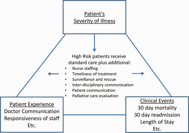
Clinicians may not typically compartmentalize what they do to improve outcomes versus the patient experience. A possible source for new improvement strategies is to understand the types of patients in which both adverse outcomes and suboptimal experiences are likely to occur, then redesign the multidisciplinary care processes to address both concurrently.[7] Previous studies support the existence of a relationship between a higher mortality risk on admission and subsequent worse outcomes, as well as a relationship between worse outcomes and lower HCAHPS scores.[8, 9, 10, 11, 12, 13] We hypothesized the mortality risk on admission, patient experience, and outcomes might share a triad relationship (Figure 1). In this article we explore the third edge of this triangle, the association between the mortality risk on admission and the subsequent patient experience.
METHODS
We studied HCAHPS from 5 midwestern US hospitals having 113, 136, 304, 443, and 537 licensed beds, affiliated with the same multistate healthcare system. HCAHPS telephone surveys were administered via a vendor to a random sample of inpatients 18 years of age or older discharged from January 1, 2012 through June 30, 2014. Per CMS guidelines, surveyed patients must have been discharged alive after a hospital stay of at least 1 night.[14] Patients ineligible to be surveyed included those discharged to skilled nursing facilities or hospice care.[14] Because not all study hospitals provided obstetrical services, we restricted the analyses to medical and surgical respondents. With the permission of the local institutional review board, subjects' survey responses were linked confidentially to their clinical data.
We focused on the 8 dimensions of the care experience used in the CMS Value Based Purchasing program: communication with doctors, communication with nurses, responsiveness of hospital staff, pain management, communication about medicines, discharge information, hospital environment, and an overall rating of the hospital.[2] Following the scoring convention for publicly reported results, we dichotomized the 4‐level Likert scales into the most favorable response possible (always) versus all other responses.[15] Similarly we dichotomized the hospital rating scale at 9 and above for the most favorable response.
Our unit of analysis was an individual hospitalization. Our primary outcome of interest was whether or not the respondent provided the most favorable response for all questions answered within a given domain. For example, for the physician communication domain, the patient must have answered always to each of the 3 questions answered within the domain. This approach is appropriate for learning which patient‐level factors influence the survey responses, but differs from that used for the publically reported domain scores for which the relative performance of hospitals is the focus.[16] For the latter, the hospital was the unit of analysis, and the domain score was basically the average of the percentages of top box scores for the questions within a domain. For example, if 90% respondents from a hospital provided a top box response for courtesy, 80% for listening, and 70% for explanation, the hospital's physician communication score would be (90 + 80 + 70)/3 = 80%.[17]
Our primary explanatory variable was a binary high versus low mortality‐risk status of the respondent on admission based on age, gender, prior hospitalizations, clinical laboratory values, and diagnoses present on admission.[12] The calculated mortality risk was then dichotomized prior to the analysis at a probability of dying equal to 0.07 or higher. This corresponded roughly to the top quintile of predicted risk found in prior studies.[12, 13] During the study period, only 2 of the hospitals had the capability of generating mortality scores in real time, so for this study the mortality risk was calculated retrospectively, using information deemed present on admission.[12]
To estimate the sample size, we assumed that the high‐risk strata contained approximately 13% of respondents, and that the true percent of top box responses from patients in the lower‐risk stratum was approximately 80% for each domain. A meaningful difference in the proportion of most favorable responses was considered as an odds ratio (OR) of 0.75 for high risk versus low risk. A significance level of P 0.003 was set to control study‐wide type I error due to multiple comparisons. We determined that for each dimension, approximately 8583 survey responses would be required for low‐risk patients and approximately 1116 responses for high‐risk patients to achieve 80% power under these assumptions. We were able to accrue the target number of surveys for all but 3 domains (pain management, communication about medicines, and hospital environment) because of data availability, and because patients are allowed to skip questions that do not apply. Univariate relationships were examined with 2, t test, and Fisher exact tests where indicated. Generalized linear mixed regression models with a logit link were fit to determine the association between patient mortality risk and the top box experience for each of the HCAHPS domains and for the overall rating. The patient's hospital was considered a random intercept to account for the patient‐hospital hierarchy and the unmeasured hospital‐specific practices. The multivariable models controlled for gender plus the HCAHPS patient‐mix adjustment variables of age, education, self‐rated health, language spoken at home, service line, and the number of days elapsed between the date of discharge and date of the survey.[18, 19, 20, 21] In keeping with the industry analyses, a second order interaction variable was included between surgery patients and age.[19] We considered the potential collinearity between the mortality risk status, age, and patient self‐reported health. We found the variance inflation factors were small, so we drew inference from the full multivariable model.
We also performed a post hoc sensitivity analysis to determine if our conclusions were biased due to missing patient responses for the risk‐adjustment variables. Accordingly, we imputed the response level most negatively associated with most HCAHPS domains as previously reported and reran the multivariable models.[19] We did not find a meaningful change in our conclusions (see Supporting Figure 1 in the online version of this article).
RESULTS
The hospitals discharged 152,333 patients during the study period, 39,905 of whom (26.2 %) had a predicted 30‐day mortality risk greater or equal to 0.07 (Table 1). Of the 36,280 high‐risk patients discharged alive, 5901 (16.3%) died in the ensuing 30 days, and 7951 (22%) were readmitted.
| Characteristic | Low‐Risk Stratum, No./Discharged (%) or Mean (SD) | High‐Risk Stratum, No./Discharged (%) or Mean (SD) | P Value* |
|---|---|---|---|
| |||
| Total discharges (row percent) | 112,428/152,333 (74) | 39,905/152,333 (26) | 0.001 |
| Total alive discharges (row percent) | 111,600/147,880 (75) | 36,280/147,880 (25) | 0.001 |
| No. of respondents (row percent) | 14,996/17,509 (86) | 2,513/17,509 (14) | |
| HCAHPS surveys completed | 14,996/111,600 (13) | 2,513/36,280 (7) | 0.001 |
| Readmissions within 30 days (total discharges) | 12,311/112,428 (11) | 7,951/39,905 (20) | 0.001 |
| Readmissions within 30 days (alive discharges) | 12,311/111,600 (11) | 7,951/36,280 (22) | 0.001 |
| Readmissions within 30 days (respondents) | 1,220/14,996 (8) | 424/2,513 (17) | 0.001 |
| Mean predicted probability of 30‐day mortality (total discharges) | 0.022 (0.018) | 0.200 (0.151) | 0.001 |
| Mean predicted probability of 30‐day mortality (alive discharges) | 0.022 (0.018) | 0.187 (0.136) | 0.001 |
| Mean predicted probability of 30‐day mortality (respondents) | 0.020 (0.017) | 0.151 (0.098) | 0.001 |
| In‐hospital death (total discharges) | 828/112,428 (0.74) | 3,625/39,905 (9) | 0.001 |
| Mortality within 30 days (total discharges) | 2,455/112,428 (2) | 9,526/39,905 (24) | 0.001 |
| Mortality within 30 days (alive discharges) | 1,627/111,600 (1.5) | 5,901/36,280 (16) | 0.001 |
| Mortality within 30 days (respondents) | 9/14,996 (0.06) | 16/2,513 (0.64) | 0.001 |
| Female (total discharges) | 62,681/112,368 (56) | 21,058/39,897 (53) | 0.001 |
| Female (alive discharges) | 62,216/111,540 (56) | 19,164/36,272 (53) | 0.001 |
| Female (respondents) | 8,684/14,996 (58) | 1,318/2,513 (52) | 0.001 |
| Age (total discharges) | 61.3 (16.8) | 78.3 (12.5) | 0.001 |
| Age (alive discharges) | 61.2 (16.8) | 78.4 (12.5) | 0.001 |
| Age (respondents) | 63.1 (15.2) | 76.6 (11.5) | 0.001 |
| Highest education attained | |||
| 8th grade or less | 297/14,996 (2) | 98/2,513 (4) | |
| Some high school | 1,190/14,996 (8) | 267/2,513 (11) | |
| High school grad | 4,648/14,996 (31) | 930/2,513 (37) | 0.001 |
| Some college | 6,338/14,996 (42) | 768/2,513 (31) | |
| 4‐year college grad | 1,502/14,996 (10) | 183/2,513 (7) | |
| Missing response | 1,021/14,996 (7) | 267/2,513 (11) | |
| Language spoken at home | |||
| English | 13,763/14,996 (92) | 2,208/2,513 (88) | |
| Spanish | 56/14,996 (0.37) | 8/2,513 (0.32) | 0.47 |
| Chinese | 153/14,996 (1) | 31/2,513 (1) | |
| Missing response | 1,024/14,996 (7) | 266/2,513 (11) | |
| Self‐rated health | |||
| Excellent | 1,399/14,996 (9) | 114/2,513 (5) | |
| Very good | 3,916/14,996 (26) | 405/2,513 (16) | |
| Good | 4,861/14,996 (32) | 713/2,513 (28) | |
| Fair | 2,900/14,996 (19) | 652/2,513 (26) | 0.001 |
| Poor | 1,065/14,996 (7) | 396/2,513 (16) | |
| Missing response | 855/14,996 (6) | 233/2,513 (9) | |
| Length of hospitalization, d (respondents) | 3.5 (2.8) | 4.6 (3.6) | 0.001 |
| Consulting specialties (respondents) | 1.7 (1.0) | 2.2 (1.3) | 0.001 |
| Service line | |||
| Surgical | 6,380/14,996 (43) | 346/2,513 (14) | 0.001 |
| Medical | 8,616/14,996 (57) | 2,167/2,513 (86) | |
| HCAHPS | |||
| Domain 1: Communication With Doctors | 9,564/14,731 (65) | 1,339/2,462 (54) | 0.001 |
| Domain 2: Communication With Nurses | 10,097/14,991 (67) | 1,531/2,511 (61) | 0.001 |
| Domain 3: Responsiveness of Hospital Staff | 7,813/12,964 (60) | 1,158/2,277 (51) | 0.001 |
| Domain 4: Pain Management | 6,565/10,424 (63) | 786/1,328 (59) | 00.007 |
| Domain 5: Communication About Medicines | 3,769/8,088 (47) | 456/1,143 (40) | 0.001 |
| Domain 6: Discharge Information | 11,331/14,033 (81) | 1,767/2,230 (79) | 0.09 |
| Domain 7: Hospital Environment | 6,981/14,687 (48) | 1,093/2,451 (45) | 0.007 |
| Overall rating | 10,708/14,996 (71) | 1,695/2,513 (67) | 0.001 |
The high‐risk subset was under‐represented in those who completed the HCAHPS survey with 7% (2513/36,280) completing surveys compared to 13% of low‐risk patients (14,996/111,600) (P 0.0001). Moreover, compared to high‐risk patients who were alive at discharge but did not complete surveys, high‐risk survey respondents were less likely to die within 30 days (16/2513 = 0.64% vs 5885/33,767 = 17.4%, P 0.0001), and less likely to be readmitted (424/2513 = 16.9% vs 7527/33,767 = 22.3%, P 0.0001).
On average, high‐risk respondents (compared to low risk) were slightly less likely to be female (52.4% vs 57.9%), less educated (30.6% with some college vs 42.3%), less likely to have been on a surgical service (13.8% vs 42.5%), and less likely to report good or better health (49.0% vs 68.0%, all P 0.0001). High‐risk respondents were also older (76.6 vs 63.1 years), stayed in the hospital longer (4.6 vs 3.5 days), and received care from more specialties (2.2 vs 1.7 specialties) (all P 0.0001). High‐risk respondents experienced more 30‐day readmissions (16.9% vs 8.1%) and deaths within 30 days (0.6 % vs 0.1 %, all P 0.0001) than their low‐risk counterparts.
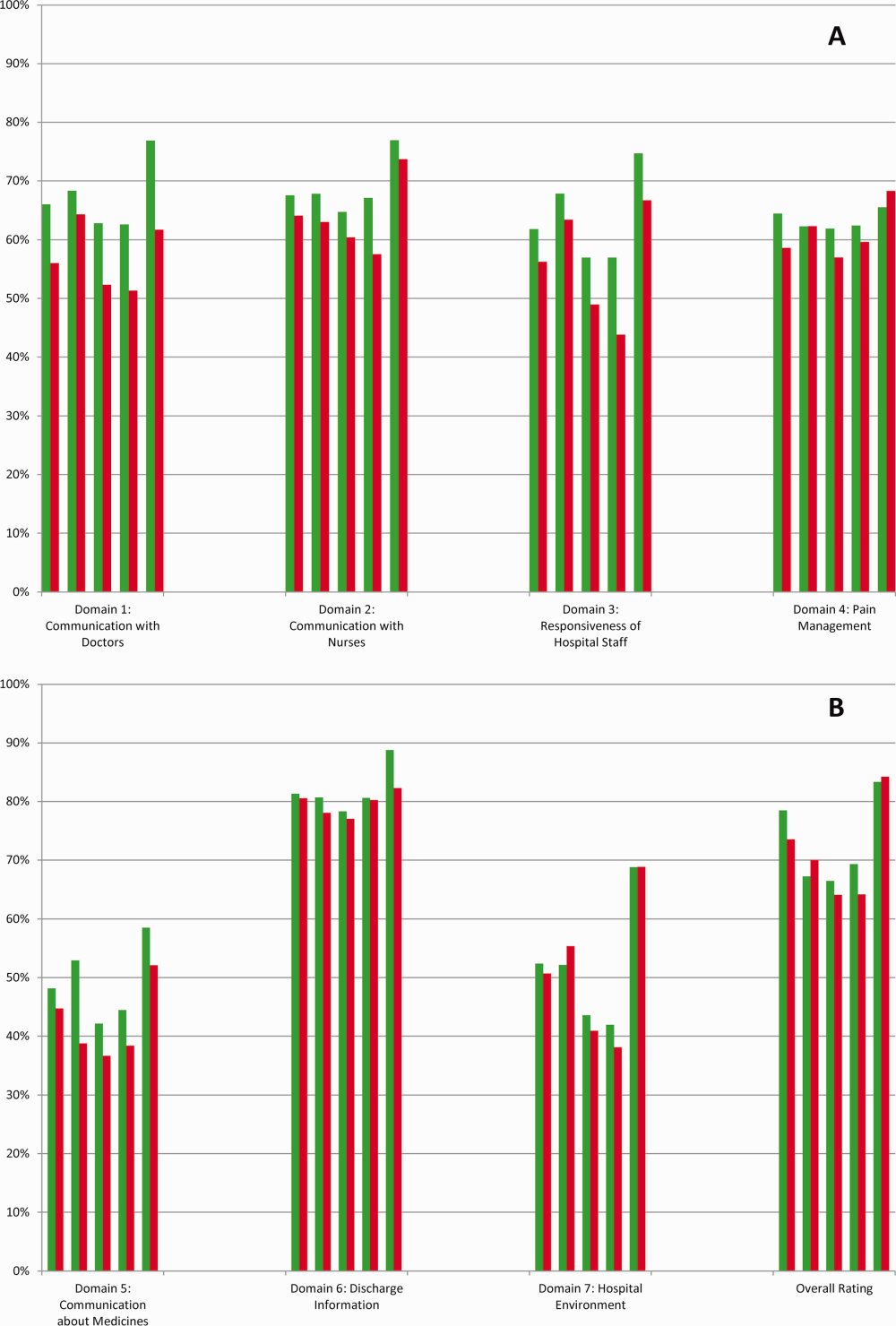
High‐risk respondents were less likely to provide the most favorable response (unadjusted) for all HCAHPS domains compared to low‐risk respondents, although the difference was not significant for discharge information (Table 1, Figure 2A). The gradient between high‐risk and low‐risk patients was seen for all domains within each hospital except for pain management, hospital environment, and overall rating (Figure 3).
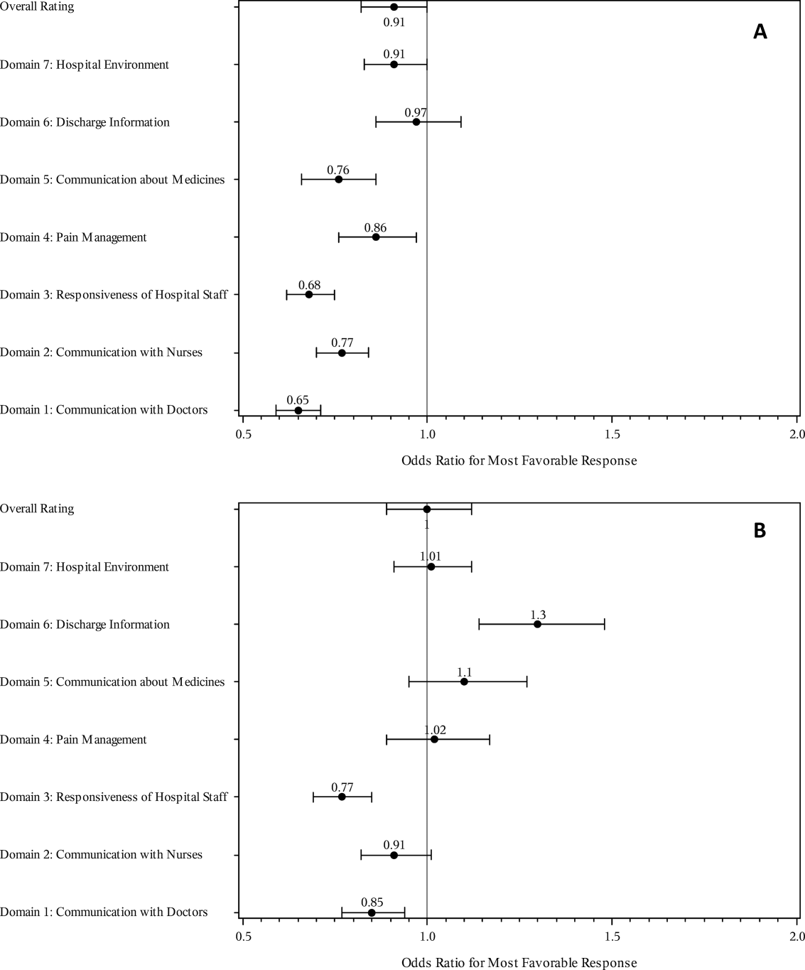
The multivariable regression models examined whether the mortality risk on admission simply represented older medical patients and/or those who considered themselves unhealthy (Figure 2B) (see Supporting Table 1 in the online version of this article). Accounting for hospital, age, gender, language, self‐reported health, educational level, service line, and days elapsed from discharge, respondents in the high‐mortality‐risk stratum were still less likely to report an always experience for doctor communication (OR: 0.85; 95% confidence interval [CI]: 0.77‐0.94) and responsiveness of hospital staff (OR: 0.77; 95% CI: 0.69‐0.85). Higher‐risk patients also tended to have less favorable experiences with nursing communication, although the CI crossed 1 (OR: 0.91; 95% CI: 0.82‐1.01). In contrast, higher‐risk patients were more likely to provide top box responses for having received discharge information (OR: 1.30; 95% CI: 1.14‐1.48). We did not find independent associations between mortality risk and the other domains when the patient risk‐adjustment factors were considered.[18, 19, 20, 21]
DISCUSSION
The high‐mortality‐risk stratum on admission contained a subset of patients who provided less favorable responses for almost all incentivized HCAHPS domains when other risk‐adjustment variables were not taken into consideration (Figure 2A). These univariate relationships weakened when we controlled for gender, the standard HCAHPS risk‐adjustment variables, and individual hospital influences (Figure 2B).[18, 19, 20, 21] After multivariable adjustment, survey respondents in the high‐risk category remained less likely to report their physicians always communicated well and to experience hospital staff responding quickly, but were more likely to report receiving discharge information. We did not find an independent association between the underlying mortality risk and the other incentivized HCAHPS domains after risk adjustment.
We are cautious with initial interpretations of our findings in light of the relatively small number of hospitals studied and the substantial survey response bias of healthier patients. Undoubtedly, the CMS exclusions of patients discharged to hospice or skilled nursing facilities provide a partial explanation for the selection bias, but the experience of those at high risk who did not complete surveys remains conjecture at this point.[14] Previous evidence suggests sicker patients and those with worse experiences are less likely to respond to the HCAHPS survey.[18, 22] On the other hand, it is possible that high‐risk nonrespondents who died could have received better communication and staff responsiveness.[23, 24] We were unable to find a previous, patient‐level study that explicitly tested the association between the admission mortality risk and the subsequent patient experience, yet our findings are consistent with a previous single‐site study of a surgical population showing lower overall ratings from patients with higher Injury Severity Scores.[25]
Our findings provide evidence of complex relationships among admission mortality risk, the 3 domains of the patient experience, and adverse outcomes, at least within the study hospitals (Figure 1). The developing field of palliative care has found very ill patients have special communication needs regarding goals of care, as well as physical symptoms, anxiety, and depression that might prompt more calls for help.[26] If these needs were more important for high‐risk compared to low‐risk patients, and were either not recognized or adequately addressed by the clinical teams at the study hospitals, then the high‐risk patients may have been less likely to perceive their physicians listened and explained things well, or that staff responded promptly to their requests for help.[27] On the other hand, the higher ratings for discharge information suggest the needs of the high‐risk patients were relatively easier to address by current practices at these hospitals. The lack of association between the mortality risk and the other HCAHPS domains may reflect the relatively stronger influence of age, gender, educational level, provider variability, and other unmeasured influences within the study sites, or that the level of patient need was similar among high‐risk and low‐risk patients within these domains.[27]
There are several possible confounders of our observed relationship between mortality risk and HCAHPS scores. The first category of confounders represents patient level variables that might impact the communication scores, some of which are part of the formula of our mortality prediction rule, for example, cognitive impairment and emergent admission.[18, 22, 27] The effect of the mortality risk could also be confounded by unmeasured patient‐level factors such as lower socioeconomic status.[28] A second category of confounders pertains to clinical outcomes and processes of care associated with serious illness irrespective of the risk of dying. More physicians involved in the care of the seriously ill (Table 1) may impact the communication scores, due to the larger opportunity for conflicting or confusing information presented to patients and their families.[29] The longer hospital stays, readmissions, and adverse events of the seriously ill may also underlie the apparent association between mortality risk and HCAHPS scores.[8, 9, 10]
Even if we do not understand precisely if and how the mortality risk might be associated with suboptimal physician communication and staff responsiveness, there may still be some value in considering how these possible relationships could be leveraged to improve patient care. We recall Berwick's insight that every system is perfectly designed to achieve the results it achieves.[7] We have previously argued for the use of mortality‐risk strata to initiate concurrent, multidisciplinary care processes to reduce adverse outcomes.[12, 13] Others have used risk‐based approaches for anticipating clinical deterioration of surgical patients, and determining the intensity of individualized case management services.[30, 31] In this framework, all patients receive a standard set of care processes, but higher‐risk patients receive additional efforts to promote better outcomes. An efficient extension of this approach is to assume patients at risk for adverse outcomes also have additional needs for communication, coordination of specialty care, and timely response to the call button. The admission mortality risk could be used as a determinant for the level of nurse staffing to reduce deaths plus shorten response time to the call button.[32, 33] Hospitalists and specialists could work together on a standard way to conference among themselves for high‐risk patients above that needed for less‐complex cases. Patients in the high‐risk strata could be screened early to see if they might benefit from the involvement of the palliative care team.[26]
Our study has limitations in addition to those already noted. First, our use of the top box as the formulation of the outcome of interest could be challenged. We chose this to be relevant to the Value‐Based Purchasing environment, but other formulations or use of other survey instruments may be needed to tease out the complex relationships we hypothesize. Next, we do not know the extent to which the patients and care processes reflected in our study represent other settings. The literature indicates some hospitals are more effective in providing care for certain subgroups of patients than for others, and that there is substantial regional variation in care intensity that is in turn associated with the patient experience.[29, 34] The mortality‐risk experience relationship for nonstudy hospitals could be weaker or stronger than what we found. Third, many hospitals may not have the capability to generate mortality scores on admission, although more hospitals may be able to do so in the future.[35] Explicit risk strata have the benefit of providing members of the multidisciplinary team with a quick preview of the clinical needs and prognoses of patients in much the way that the term baroque alerts the audience to the genre of music. Still, clinicians in any hospital could attempt to improve outcomes and experience through the use of informal risk assessment during interdisciplinary care rounds or by simply asking the team if they would be surprised if this patient died in the next year.[30, 36] Finally, we do not know if awareness of an experience risk will identify remediable practices that actually improve the experience. Clearly, future studies are needed to answer all of these concerns.
We have provided evidence that a group of patients who were at elevated risk for dying at the time of admission were more likely to have issues with physician communication and staff responsiveness than their lower‐risk counterparts. While we await future studies to confirm these findings, clinical teams can consider whether or not their patients' HCAHPS scores reflect how their system of care addresses the needs of these vulnerable people.
Acknowledgements
The authors thank Steven Lewis for assistance in the interpretation of the HCAHPS scores, Bonita Singal, MD, PhD, for initial statistical consultation, and Frank Smith, MD, for reviewing an earlier version of the manuscript. The authors acknowledge the input of the peer reviewers.
Disclosures: Dr. Cowen and Mr. Kabara had full access to all of the data in the study and take responsibility for the integrity of the data and the accuracy of the data analysis. Study concept and design: all authors. Acquisition, analysis or interpretation of data: all authors. Drafting of the manuscript: Dr. Cowen and Mr. Kabara. Critical revision of the manuscript for important intellectual content: all authors. Statistical analysis: Dr. Cowen and Mr. Kabara. Administrative, technical or material support: Ms. Czerwinski. Study supervision: Dr. Cowen and Ms. Czerwinski. Funding/support: internal. Conflicts of interest disclosures: no potential conflicts reported.
Disclosures
Dr. Cowen and Mr. Kabara had full access to all of the data in the study and take responsibility for the integrity of the data and the accuracy of the data analysis. Study concept and design: all authors. Acquisition, analysis or interpretation of data: all authors. Drafting of the manuscript: Dr. Cowen and Mr. Kabara. Critical revision of the manuscript for important intellectual content: all authors. Statistical analysis: Dr. Cowen and Mr. Kabara. Administrative, technical or material support: Ms. Czerwinski. Study supervision: Dr. Cowen and Ms. Czerwinski. Funding/support: internal. Conflicts of interest disclosures: no potential conflicts reported.
- , , , , . Measuring hospital care from the patients' perspective: an overview of the CAHPS hospital survey development process. Health Serv Res. 2005;40 (6 part 2):1977–1995.
- Centers for Medicare 79(163):49854–50449.
- , , , . The relationship between patients' perception of care and measures of hospital quality and safety. Health Serv Res. 2010;45(4):1024–1040.
- Centers for Medicare 312(7031):619–622.
- , , , , . Relationship between patient satisfaction with inpatient care and hospital readmission within 30 days. Am J Manag Care. 2011;17(1):41–48.
- , , , , , . Getting satisfaction: drivers of surgical Hospital Consumer Assessment of Health care Providers and Systems survey scores. J Surg Res. 2015;197(1):155–161.
- , , . Patient satisfaction and quality of surgical care in US hospitals. Ann Surg. 2015;261(1):2–8.
- , , . Is there a relationship between patient satisfaction and favorable outcomes? Ann Surg. 2014;260(4):592–598; discussion 598–600.
- , , , , . Mortality predictions on admission as a context for organizing care activities. J Hosp Med. 2013;8(5):229–235.
- , , , et al. Implementation of a mortality prediction rule for real‐time decision making: feasibility and validity. J Hosp Med. 2014;9(11):720–726.
- Centers for Medicare 40(6 pt 2):2078–2095.
- Centers for Medicare 44(2 pt 1):501–518.
- Patient‐mix coefficients for October 2015 (1Q14 through 4Q14 discharges) publicly reported HCAHPS Results. Available at: http://www.hcahpsonline.org/Files/October_2015_PMA_Web_Document_a.pdf. Published July 2, 2015. Accessed August 4, 2015.
- , , , , . Case‐mix adjustment of the CAHPS hospital survey. Health Serv Res. 2005;40(6):2162–2181.
- , , , et.al. Gender differences in patients' perceptions of inpatient care. Health Serv Res. 2012;47(4):1482–1501.
- , , , et al. Patterns of unit and item nonresponse in the CAHPS hospital survey. Health Serv Res. 2005;40(6 pt 2):2096–2119.
- , , , . The cost of satisfaction: a national study of patient satisfaction, health care utilization, expenditures, and mortality. Arch Intern Med. 2012;172(5):405–411.
- , , , et al. Care experiences of managed care Medicare enrollees near the end of life. J Am Geriatr Soc. 2013;61(3):407–412.
- , , , , . Measuring satisfaction: factors that drive hospital consumer assessment of healthcare providers and systems survey responses in a trauma and acute care surgery population. Am Surg. 2015;81(5):537–543.
- , . Palliative care for the seriously ill. N Engl J Med. 2015;373(8):747–755.
- , , , et.al. Components of care vary in importance for overall patient‐reported experience by type of hospitalization. Med Care. 2009;47(8):842–849.
- , , , et al. Socioeconomic status, structural and functional measures of social support, and mortality: the British Whitehall II cohort study, 1985–2009. Am J Epidemiol. 2012;175(12):1275–1283.
- , , , et al. Inpatient care intensity and patients' ratings of their hospital experiences. Health Aff (Millwood). 2009;28(1):103–112.
- , , , et al. A validated value‐based model to improve hospital‐wide perioperative outcomes. Ann Surg. 2010;252(3):486–498.
- , , , et al. Allocating scare resources in real‐time to reduce heart failure readmissions: a prospective, controlled study. BMJ Qual Saf. 2013;22(12):998–1005.
- , , , . Patients' perception of hospital care in the United States. N Engl J Med. 2008;359(18):1921–1931.
- , , , , , . Nurse staffing and inpatient hospital mortality. N Engl J Med. 2011;364(11):1037–1045.
- , , , et al. Do hospitals rank differently on HCAHPS for different patient subgroups? Med Care Res Rev. 2010;67(1):56–73.
- , , , , , . Risk‐adjusting hospital inpatient mortality using automated inpatient, outpatient, and laboratory databases. Med Care. 2008;46(3):232–239.
- , , , et al. Utility of the “surprise” question to identify dialysis patients with high mortality. Clin J Am Soc Nephrol. 2008;3(5):1379–1384.
Few today deny the importance of the Hospital Consumer Assessment of Healthcare Providers and Systems (HCAHPS) survey.[1, 2] The Centers for Medicare and Medicaid Services' (CMS) Value Based Purchasing incentive, sympathy for the ill, and relationships between the patient experience and quality of care provide sufficient justification.[3, 4] How to improve the experience scores is not well understood. The national scores have improved only modestly over the past 3 years.[5, 6]
Clinicians may not typically compartmentalize what they do to improve outcomes versus the patient experience. A possible source for new improvement strategies is to understand the types of patients in which both adverse outcomes and suboptimal experiences are likely to occur, then redesign the multidisciplinary care processes to address both concurrently.[7] Previous studies support the existence of a relationship between a higher mortality risk on admission and subsequent worse outcomes, as well as a relationship between worse outcomes and lower HCAHPS scores.[8, 9, 10, 11, 12, 13] We hypothesized the mortality risk on admission, patient experience, and outcomes might share a triad relationship (Figure 1). In this article we explore the third edge of this triangle, the association between the mortality risk on admission and the subsequent patient experience.
METHODS
We studied HCAHPS from 5 midwestern US hospitals having 113, 136, 304, 443, and 537 licensed beds, affiliated with the same multistate healthcare system. HCAHPS telephone surveys were administered via a vendor to a random sample of inpatients 18 years of age or older discharged from January 1, 2012 through June 30, 2014. Per CMS guidelines, surveyed patients must have been discharged alive after a hospital stay of at least 1 night.[14] Patients ineligible to be surveyed included those discharged to skilled nursing facilities or hospice care.[14] Because not all study hospitals provided obstetrical services, we restricted the analyses to medical and surgical respondents. With the permission of the local institutional review board, subjects' survey responses were linked confidentially to their clinical data.
We focused on the 8 dimensions of the care experience used in the CMS Value Based Purchasing program: communication with doctors, communication with nurses, responsiveness of hospital staff, pain management, communication about medicines, discharge information, hospital environment, and an overall rating of the hospital.[2] Following the scoring convention for publicly reported results, we dichotomized the 4‐level Likert scales into the most favorable response possible (always) versus all other responses.[15] Similarly we dichotomized the hospital rating scale at 9 and above for the most favorable response.
Our unit of analysis was an individual hospitalization. Our primary outcome of interest was whether or not the respondent provided the most favorable response for all questions answered within a given domain. For example, for the physician communication domain, the patient must have answered always to each of the 3 questions answered within the domain. This approach is appropriate for learning which patient‐level factors influence the survey responses, but differs from that used for the publically reported domain scores for which the relative performance of hospitals is the focus.[16] For the latter, the hospital was the unit of analysis, and the domain score was basically the average of the percentages of top box scores for the questions within a domain. For example, if 90% respondents from a hospital provided a top box response for courtesy, 80% for listening, and 70% for explanation, the hospital's physician communication score would be (90 + 80 + 70)/3 = 80%.[17]
Our primary explanatory variable was a binary high versus low mortality‐risk status of the respondent on admission based on age, gender, prior hospitalizations, clinical laboratory values, and diagnoses present on admission.[12] The calculated mortality risk was then dichotomized prior to the analysis at a probability of dying equal to 0.07 or higher. This corresponded roughly to the top quintile of predicted risk found in prior studies.[12, 13] During the study period, only 2 of the hospitals had the capability of generating mortality scores in real time, so for this study the mortality risk was calculated retrospectively, using information deemed present on admission.[12]
To estimate the sample size, we assumed that the high‐risk strata contained approximately 13% of respondents, and that the true percent of top box responses from patients in the lower‐risk stratum was approximately 80% for each domain. A meaningful difference in the proportion of most favorable responses was considered as an odds ratio (OR) of 0.75 for high risk versus low risk. A significance level of P 0.003 was set to control study‐wide type I error due to multiple comparisons. We determined that for each dimension, approximately 8583 survey responses would be required for low‐risk patients and approximately 1116 responses for high‐risk patients to achieve 80% power under these assumptions. We were able to accrue the target number of surveys for all but 3 domains (pain management, communication about medicines, and hospital environment) because of data availability, and because patients are allowed to skip questions that do not apply. Univariate relationships were examined with 2, t test, and Fisher exact tests where indicated. Generalized linear mixed regression models with a logit link were fit to determine the association between patient mortality risk and the top box experience for each of the HCAHPS domains and for the overall rating. The patient's hospital was considered a random intercept to account for the patient‐hospital hierarchy and the unmeasured hospital‐specific practices. The multivariable models controlled for gender plus the HCAHPS patient‐mix adjustment variables of age, education, self‐rated health, language spoken at home, service line, and the number of days elapsed between the date of discharge and date of the survey.[18, 19, 20, 21] In keeping with the industry analyses, a second order interaction variable was included between surgery patients and age.[19] We considered the potential collinearity between the mortality risk status, age, and patient self‐reported health. We found the variance inflation factors were small, so we drew inference from the full multivariable model.
We also performed a post hoc sensitivity analysis to determine if our conclusions were biased due to missing patient responses for the risk‐adjustment variables. Accordingly, we imputed the response level most negatively associated with most HCAHPS domains as previously reported and reran the multivariable models.[19] We did not find a meaningful change in our conclusions (see Supporting Figure 1 in the online version of this article).
RESULTS
The hospitals discharged 152,333 patients during the study period, 39,905 of whom (26.2 %) had a predicted 30‐day mortality risk greater or equal to 0.07 (Table 1). Of the 36,280 high‐risk patients discharged alive, 5901 (16.3%) died in the ensuing 30 days, and 7951 (22%) were readmitted.
| Characteristic | Low‐Risk Stratum, No./Discharged (%) or Mean (SD) | High‐Risk Stratum, No./Discharged (%) or Mean (SD) | P Value* |
|---|---|---|---|
| |||
| Total discharges (row percent) | 112,428/152,333 (74) | 39,905/152,333 (26) | 0.001 |
| Total alive discharges (row percent) | 111,600/147,880 (75) | 36,280/147,880 (25) | 0.001 |
| No. of respondents (row percent) | 14,996/17,509 (86) | 2,513/17,509 (14) | |
| HCAHPS surveys completed | 14,996/111,600 (13) | 2,513/36,280 (7) | 0.001 |
| Readmissions within 30 days (total discharges) | 12,311/112,428 (11) | 7,951/39,905 (20) | 0.001 |
| Readmissions within 30 days (alive discharges) | 12,311/111,600 (11) | 7,951/36,280 (22) | 0.001 |
| Readmissions within 30 days (respondents) | 1,220/14,996 (8) | 424/2,513 (17) | 0.001 |
| Mean predicted probability of 30‐day mortality (total discharges) | 0.022 (0.018) | 0.200 (0.151) | 0.001 |
| Mean predicted probability of 30‐day mortality (alive discharges) | 0.022 (0.018) | 0.187 (0.136) | 0.001 |
| Mean predicted probability of 30‐day mortality (respondents) | 0.020 (0.017) | 0.151 (0.098) | 0.001 |
| In‐hospital death (total discharges) | 828/112,428 (0.74) | 3,625/39,905 (9) | 0.001 |
| Mortality within 30 days (total discharges) | 2,455/112,428 (2) | 9,526/39,905 (24) | 0.001 |
| Mortality within 30 days (alive discharges) | 1,627/111,600 (1.5) | 5,901/36,280 (16) | 0.001 |
| Mortality within 30 days (respondents) | 9/14,996 (0.06) | 16/2,513 (0.64) | 0.001 |
| Female (total discharges) | 62,681/112,368 (56) | 21,058/39,897 (53) | 0.001 |
| Female (alive discharges) | 62,216/111,540 (56) | 19,164/36,272 (53) | 0.001 |
| Female (respondents) | 8,684/14,996 (58) | 1,318/2,513 (52) | 0.001 |
| Age (total discharges) | 61.3 (16.8) | 78.3 (12.5) | 0.001 |
| Age (alive discharges) | 61.2 (16.8) | 78.4 (12.5) | 0.001 |
| Age (respondents) | 63.1 (15.2) | 76.6 (11.5) | 0.001 |
| Highest education attained | |||
| 8th grade or less | 297/14,996 (2) | 98/2,513 (4) | |
| Some high school | 1,190/14,996 (8) | 267/2,513 (11) | |
| High school grad | 4,648/14,996 (31) | 930/2,513 (37) | 0.001 |
| Some college | 6,338/14,996 (42) | 768/2,513 (31) | |
| 4‐year college grad | 1,502/14,996 (10) | 183/2,513 (7) | |
| Missing response | 1,021/14,996 (7) | 267/2,513 (11) | |
| Language spoken at home | |||
| English | 13,763/14,996 (92) | 2,208/2,513 (88) | |
| Spanish | 56/14,996 (0.37) | 8/2,513 (0.32) | 0.47 |
| Chinese | 153/14,996 (1) | 31/2,513 (1) | |
| Missing response | 1,024/14,996 (7) | 266/2,513 (11) | |
| Self‐rated health | |||
| Excellent | 1,399/14,996 (9) | 114/2,513 (5) | |
| Very good | 3,916/14,996 (26) | 405/2,513 (16) | |
| Good | 4,861/14,996 (32) | 713/2,513 (28) | |
| Fair | 2,900/14,996 (19) | 652/2,513 (26) | 0.001 |
| Poor | 1,065/14,996 (7) | 396/2,513 (16) | |
| Missing response | 855/14,996 (6) | 233/2,513 (9) | |
| Length of hospitalization, d (respondents) | 3.5 (2.8) | 4.6 (3.6) | 0.001 |
| Consulting specialties (respondents) | 1.7 (1.0) | 2.2 (1.3) | 0.001 |
| Service line | |||
| Surgical | 6,380/14,996 (43) | 346/2,513 (14) | 0.001 |
| Medical | 8,616/14,996 (57) | 2,167/2,513 (86) | |
| HCAHPS | |||
| Domain 1: Communication With Doctors | 9,564/14,731 (65) | 1,339/2,462 (54) | 0.001 |
| Domain 2: Communication With Nurses | 10,097/14,991 (67) | 1,531/2,511 (61) | 0.001 |
| Domain 3: Responsiveness of Hospital Staff | 7,813/12,964 (60) | 1,158/2,277 (51) | 0.001 |
| Domain 4: Pain Management | 6,565/10,424 (63) | 786/1,328 (59) | 00.007 |
| Domain 5: Communication About Medicines | 3,769/8,088 (47) | 456/1,143 (40) | 0.001 |
| Domain 6: Discharge Information | 11,331/14,033 (81) | 1,767/2,230 (79) | 0.09 |
| Domain 7: Hospital Environment | 6,981/14,687 (48) | 1,093/2,451 (45) | 0.007 |
| Overall rating | 10,708/14,996 (71) | 1,695/2,513 (67) | 0.001 |
The high‐risk subset was under‐represented in those who completed the HCAHPS survey with 7% (2513/36,280) completing surveys compared to 13% of low‐risk patients (14,996/111,600) (P 0.0001). Moreover, compared to high‐risk patients who were alive at discharge but did not complete surveys, high‐risk survey respondents were less likely to die within 30 days (16/2513 = 0.64% vs 5885/33,767 = 17.4%, P 0.0001), and less likely to be readmitted (424/2513 = 16.9% vs 7527/33,767 = 22.3%, P 0.0001).
On average, high‐risk respondents (compared to low risk) were slightly less likely to be female (52.4% vs 57.9%), less educated (30.6% with some college vs 42.3%), less likely to have been on a surgical service (13.8% vs 42.5%), and less likely to report good or better health (49.0% vs 68.0%, all P 0.0001). High‐risk respondents were also older (76.6 vs 63.1 years), stayed in the hospital longer (4.6 vs 3.5 days), and received care from more specialties (2.2 vs 1.7 specialties) (all P 0.0001). High‐risk respondents experienced more 30‐day readmissions (16.9% vs 8.1%) and deaths within 30 days (0.6 % vs 0.1 %, all P 0.0001) than their low‐risk counterparts.
High‐risk respondents were less likely to provide the most favorable response (unadjusted) for all HCAHPS domains compared to low‐risk respondents, although the difference was not significant for discharge information (Table 1, Figure 2A). The gradient between high‐risk and low‐risk patients was seen for all domains within each hospital except for pain management, hospital environment, and overall rating (Figure 3).
The multivariable regression models examined whether the mortality risk on admission simply represented older medical patients and/or those who considered themselves unhealthy (Figure 2B) (see Supporting Table 1 in the online version of this article). Accounting for hospital, age, gender, language, self‐reported health, educational level, service line, and days elapsed from discharge, respondents in the high‐mortality‐risk stratum were still less likely to report an always experience for doctor communication (OR: 0.85; 95% confidence interval [CI]: 0.77‐0.94) and responsiveness of hospital staff (OR: 0.77; 95% CI: 0.69‐0.85). Higher‐risk patients also tended to have less favorable experiences with nursing communication, although the CI crossed 1 (OR: 0.91; 95% CI: 0.82‐1.01). In contrast, higher‐risk patients were more likely to provide top box responses for having received discharge information (OR: 1.30; 95% CI: 1.14‐1.48). We did not find independent associations between mortality risk and the other domains when the patient risk‐adjustment factors were considered.[18, 19, 20, 21]
DISCUSSION
The high‐mortality‐risk stratum on admission contained a subset of patients who provided less favorable responses for almost all incentivized HCAHPS domains when other risk‐adjustment variables were not taken into consideration (Figure 2A). These univariate relationships weakened when we controlled for gender, the standard HCAHPS risk‐adjustment variables, and individual hospital influences (Figure 2B).[18, 19, 20, 21] After multivariable adjustment, survey respondents in the high‐risk category remained less likely to report their physicians always communicated well and to experience hospital staff responding quickly, but were more likely to report receiving discharge information. We did not find an independent association between the underlying mortality risk and the other incentivized HCAHPS domains after risk adjustment.
We are cautious with initial interpretations of our findings in light of the relatively small number of hospitals studied and the substantial survey response bias of healthier patients. Undoubtedly, the CMS exclusions of patients discharged to hospice or skilled nursing facilities provide a partial explanation for the selection bias, but the experience of those at high risk who did not complete surveys remains conjecture at this point.[14] Previous evidence suggests sicker patients and those with worse experiences are less likely to respond to the HCAHPS survey.[18, 22] On the other hand, it is possible that high‐risk nonrespondents who died could have received better communication and staff responsiveness.[23, 24] We were unable to find a previous, patient‐level study that explicitly tested the association between the admission mortality risk and the subsequent patient experience, yet our findings are consistent with a previous single‐site study of a surgical population showing lower overall ratings from patients with higher Injury Severity Scores.[25]
Our findings provide evidence of complex relationships among admission mortality risk, the 3 domains of the patient experience, and adverse outcomes, at least within the study hospitals (Figure 1). The developing field of palliative care has found very ill patients have special communication needs regarding goals of care, as well as physical symptoms, anxiety, and depression that might prompt more calls for help.[26] If these needs were more important for high‐risk compared to low‐risk patients, and were either not recognized or adequately addressed by the clinical teams at the study hospitals, then the high‐risk patients may have been less likely to perceive their physicians listened and explained things well, or that staff responded promptly to their requests for help.[27] On the other hand, the higher ratings for discharge information suggest the needs of the high‐risk patients were relatively easier to address by current practices at these hospitals. The lack of association between the mortality risk and the other HCAHPS domains may reflect the relatively stronger influence of age, gender, educational level, provider variability, and other unmeasured influences within the study sites, or that the level of patient need was similar among high‐risk and low‐risk patients within these domains.[27]
There are several possible confounders of our observed relationship between mortality risk and HCAHPS scores. The first category of confounders represents patient level variables that might impact the communication scores, some of which are part of the formula of our mortality prediction rule, for example, cognitive impairment and emergent admission.[18, 22, 27] The effect of the mortality risk could also be confounded by unmeasured patient‐level factors such as lower socioeconomic status.[28] A second category of confounders pertains to clinical outcomes and processes of care associated with serious illness irrespective of the risk of dying. More physicians involved in the care of the seriously ill (Table 1) may impact the communication scores, due to the larger opportunity for conflicting or confusing information presented to patients and their families.[29] The longer hospital stays, readmissions, and adverse events of the seriously ill may also underlie the apparent association between mortality risk and HCAHPS scores.[8, 9, 10]
Even if we do not understand precisely if and how the mortality risk might be associated with suboptimal physician communication and staff responsiveness, there may still be some value in considering how these possible relationships could be leveraged to improve patient care. We recall Berwick's insight that every system is perfectly designed to achieve the results it achieves.[7] We have previously argued for the use of mortality‐risk strata to initiate concurrent, multidisciplinary care processes to reduce adverse outcomes.[12, 13] Others have used risk‐based approaches for anticipating clinical deterioration of surgical patients, and determining the intensity of individualized case management services.[30, 31] In this framework, all patients receive a standard set of care processes, but higher‐risk patients receive additional efforts to promote better outcomes. An efficient extension of this approach is to assume patients at risk for adverse outcomes also have additional needs for communication, coordination of specialty care, and timely response to the call button. The admission mortality risk could be used as a determinant for the level of nurse staffing to reduce deaths plus shorten response time to the call button.[32, 33] Hospitalists and specialists could work together on a standard way to conference among themselves for high‐risk patients above that needed for less‐complex cases. Patients in the high‐risk strata could be screened early to see if they might benefit from the involvement of the palliative care team.[26]
Our study has limitations in addition to those already noted. First, our use of the top box as the formulation of the outcome of interest could be challenged. We chose this to be relevant to the Value‐Based Purchasing environment, but other formulations or use of other survey instruments may be needed to tease out the complex relationships we hypothesize. Next, we do not know the extent to which the patients and care processes reflected in our study represent other settings. The literature indicates some hospitals are more effective in providing care for certain subgroups of patients than for others, and that there is substantial regional variation in care intensity that is in turn associated with the patient experience.[29, 34] The mortality‐risk experience relationship for nonstudy hospitals could be weaker or stronger than what we found. Third, many hospitals may not have the capability to generate mortality scores on admission, although more hospitals may be able to do so in the future.[35] Explicit risk strata have the benefit of providing members of the multidisciplinary team with a quick preview of the clinical needs and prognoses of patients in much the way that the term baroque alerts the audience to the genre of music. Still, clinicians in any hospital could attempt to improve outcomes and experience through the use of informal risk assessment during interdisciplinary care rounds or by simply asking the team if they would be surprised if this patient died in the next year.[30, 36] Finally, we do not know if awareness of an experience risk will identify remediable practices that actually improve the experience. Clearly, future studies are needed to answer all of these concerns.
We have provided evidence that a group of patients who were at elevated risk for dying at the time of admission were more likely to have issues with physician communication and staff responsiveness than their lower‐risk counterparts. While we await future studies to confirm these findings, clinical teams can consider whether or not their patients' HCAHPS scores reflect how their system of care addresses the needs of these vulnerable people.
Acknowledgements
The authors thank Steven Lewis for assistance in the interpretation of the HCAHPS scores, Bonita Singal, MD, PhD, for initial statistical consultation, and Frank Smith, MD, for reviewing an earlier version of the manuscript. The authors acknowledge the input of the peer reviewers.
Disclosures: Dr. Cowen and Mr. Kabara had full access to all of the data in the study and take responsibility for the integrity of the data and the accuracy of the data analysis. Study concept and design: all authors. Acquisition, analysis or interpretation of data: all authors. Drafting of the manuscript: Dr. Cowen and Mr. Kabara. Critical revision of the manuscript for important intellectual content: all authors. Statistical analysis: Dr. Cowen and Mr. Kabara. Administrative, technical or material support: Ms. Czerwinski. Study supervision: Dr. Cowen and Ms. Czerwinski. Funding/support: internal. Conflicts of interest disclosures: no potential conflicts reported.
Disclosures
Dr. Cowen and Mr. Kabara had full access to all of the data in the study and take responsibility for the integrity of the data and the accuracy of the data analysis. Study concept and design: all authors. Acquisition, analysis or interpretation of data: all authors. Drafting of the manuscript: Dr. Cowen and Mr. Kabara. Critical revision of the manuscript for important intellectual content: all authors. Statistical analysis: Dr. Cowen and Mr. Kabara. Administrative, technical or material support: Ms. Czerwinski. Study supervision: Dr. Cowen and Ms. Czerwinski. Funding/support: internal. Conflicts of interest disclosures: no potential conflicts reported.
- , , , , . Measuring hospital care from the patients' perspective: an overview of the CAHPS hospital survey development process. Health Serv Res. 2005;40 (6 part 2):1977–1995.
- Centers for Medicare 79(163):49854–50449.
- , , , . The relationship between patients' perception of care and measures of hospital quality and safety. Health Serv Res. 2010;45(4):1024–1040.
- Centers for Medicare 312(7031):619–622.
- , , , , . Relationship between patient satisfaction with inpatient care and hospital readmission within 30 days. Am J Manag Care. 2011;17(1):41–48.
- , , , , , . Getting satisfaction: drivers of surgical Hospital Consumer Assessment of Health care Providers and Systems survey scores. J Surg Res. 2015;197(1):155–161.
- , , . Patient satisfaction and quality of surgical care in US hospitals. Ann Surg. 2015;261(1):2–8.
- , , . Is there a relationship between patient satisfaction and favorable outcomes? Ann Surg. 2014;260(4):592–598; discussion 598–600.
- , , , , . Mortality predictions on admission as a context for organizing care activities. J Hosp Med. 2013;8(5):229–235.
- , , , et al. Implementation of a mortality prediction rule for real‐time decision making: feasibility and validity. J Hosp Med. 2014;9(11):720–726.
- Centers for Medicare 40(6 pt 2):2078–2095.
- Centers for Medicare 44(2 pt 1):501–518.
- Patient‐mix coefficients for October 2015 (1Q14 through 4Q14 discharges) publicly reported HCAHPS Results. Available at: http://www.hcahpsonline.org/Files/October_2015_PMA_Web_Document_a.pdf. Published July 2, 2015. Accessed August 4, 2015.
- , , , , . Case‐mix adjustment of the CAHPS hospital survey. Health Serv Res. 2005;40(6):2162–2181.
- , , , et.al. Gender differences in patients' perceptions of inpatient care. Health Serv Res. 2012;47(4):1482–1501.
- , , , et al. Patterns of unit and item nonresponse in the CAHPS hospital survey. Health Serv Res. 2005;40(6 pt 2):2096–2119.
- , , , . The cost of satisfaction: a national study of patient satisfaction, health care utilization, expenditures, and mortality. Arch Intern Med. 2012;172(5):405–411.
- , , , et al. Care experiences of managed care Medicare enrollees near the end of life. J Am Geriatr Soc. 2013;61(3):407–412.
- , , , , . Measuring satisfaction: factors that drive hospital consumer assessment of healthcare providers and systems survey responses in a trauma and acute care surgery population. Am Surg. 2015;81(5):537–543.
- , . Palliative care for the seriously ill. N Engl J Med. 2015;373(8):747–755.
- , , , et.al. Components of care vary in importance for overall patient‐reported experience by type of hospitalization. Med Care. 2009;47(8):842–849.
- , , , et al. Socioeconomic status, structural and functional measures of social support, and mortality: the British Whitehall II cohort study, 1985–2009. Am J Epidemiol. 2012;175(12):1275–1283.
- , , , et al. Inpatient care intensity and patients' ratings of their hospital experiences. Health Aff (Millwood). 2009;28(1):103–112.
- , , , et al. A validated value‐based model to improve hospital‐wide perioperative outcomes. Ann Surg. 2010;252(3):486–498.
- , , , et al. Allocating scare resources in real‐time to reduce heart failure readmissions: a prospective, controlled study. BMJ Qual Saf. 2013;22(12):998–1005.
- , , , . Patients' perception of hospital care in the United States. N Engl J Med. 2008;359(18):1921–1931.
- , , , , , . Nurse staffing and inpatient hospital mortality. N Engl J Med. 2011;364(11):1037–1045.
- , , , et al. Do hospitals rank differently on HCAHPS for different patient subgroups? Med Care Res Rev. 2010;67(1):56–73.
- , , , , , . Risk‐adjusting hospital inpatient mortality using automated inpatient, outpatient, and laboratory databases. Med Care. 2008;46(3):232–239.
- , , , et al. Utility of the “surprise” question to identify dialysis patients with high mortality. Clin J Am Soc Nephrol. 2008;3(5):1379–1384.

Choosing a Graft for Anterior Cruciate Ligament Reconstruction: Surgeon Influence Reigns Supreme
Anterior cruciate ligament (ACL) injuries affect >175,000 people each year,1 with >100,000 Americans undergoing ACL reconstruction annually.2 Due to the high impact this injury has on the general population, and especially on athletes, it is important to determine the factors that influence a patient’s selection of a particular graft type. With increasing access to information and other outside influences, surgeons should attempt to provide as much objective information as possible in order to allow patients to make appropriate informed decisions regarding their graft choice for ACL surgery.
While autografts are used in >60% of primary ACL reconstructions, allografts are used in >80% of revision procedures.3 Both autografts and allografts offer advantages and disadvantages, and the advantages of each may depend on patient age, activity level, and occupation.4 For example, graft rerupture rates have been shown to be higher in patients with ACL allografts4, while kneeling pain has been shown to be worse in patients with bone-patellar tendon-bone (BPTB) autografts compared to hamstring autografts5 as well as BPTB allografts.4
Patient satisfaction rates are high for ACL autografts and allografts. Boonriong and Kietsiriroje6 have shown visual analog scale (VAS) patient satisfaction score averages to be 88 out of 100 for BPTB autografts and 93 out of 100 for hamstring tendon autografts. Fox and colleagues7 showed that 87% of patients were completely or mostly satisfied following revision ACL reconstruction with patellar tendon allograft. Cohen and colleagues8 evaluated 240 patients undergoing primary ACL reconstruction; 63.3% underwent ACL reconstruction with an allograft and 35.4% with an autograft. Of all patients enrolled in the study, 93% were satisfied with their graft choice, with 12.7% of patients opting to choose another graft if in the same situation again. Of those patients, 63.3% would have switched from an autograft to allograft. Although these numbers represent high patient satisfaction following a variety of ACL graft types, it is important to continue to identify graft selection factors in order to maximize patient outcomes.
The purposes of this prospective study were to assess patients’ knowledge of their graft type used for ACL reconstruction, to determine the most influential factors involved in graft selection, and to determine the level of satisfaction with the graft of choice at a minimum of 1-year follow-up. Based on a previous retrospective study,8 we hypothesized that physician recommendation would be the most influential factor in ACL graft selection. We also hypothesized that patients receiving an autograft would be more accurate in stating their graft harvest location compared to allograft patients.
Materials and Methods
We prospectively enrolled 304 patients who underwent primary ACL reconstruction from January 2008 to September 2013. Surgery was performed by 9 different surgeons within the same practice. All patients undergoing primary ACL reconstruction were eligible for the study.
All surgeons explained to each patient the pros and cons of each graft choice based upon peer-reviewed literature. Each patient was allowed to choose autograft or allograft, although most of the surgeons strongly encourage patients under age 25 years to choose autograft. One of the surgeons specifically encourages a patellar tendon autograft in patients under age 30 to 35 years, except for those patients with a narrow patellar tendon on magnetic resonance imaging, in which case he recommends a hamstring autograft. Another surgeon also specifically encourages patellar tendon autograft in patients under 35 years, except in skeletally immature patients, for whom he encourages hamstring autograft. However, none of the surgeons prohibited patients from choosing autograft or allograft, regardless of age.
The Institutional Review Board at our institution provided approval for this study. At the first postoperative follow-up appointment, each patient completed a questionnaire asking to select from a list the type (“your own” or “a cadaver”) and harvest site of the graft that was used for the surgery. Patients were also asked how they decided upon that graft type by ranking a list of 4 factors from 1 to 4. These included (1) physician recommendation, (2) family/friend’s recommendation, (3) coach’s recommendation, and (4) the media. Patients had the option of ranking more than one factor as most important in their decision. In addition, patients were asked to list any other factors that influenced their decision regarding graft type.
At a minimum of 1 year following surgery, patients completed the same questionnaire described above. In addition, patients were asked if they were satisfied with their graft and whether they would choose the same graft type if undergoing ACL reconstruction again. Patients who would have chosen a different graft were asked which graft they would have chosen and why. Any patient who experienced graft rupture prior to follow-up was included in the analysis.
Statistical Analysis
Chi square tests were used to compare dichotomous outcomes. A type I error of less than 5% (P < .05) was considered statistically significant.
Results
At least 1 year following ACL reconstruction, 213 of 304 patients (70%) successfully completed the same questionnaire as they did at their first postoperative follow-up appointment. The mean age of these patients at the time of surgery was 31.9 ± 11.0 years (range, 13.9 to 58.0 years). The mean follow-up time was 1.4 ± 0.4 years (range, 1.0 to 2.6 years), and 59% of these patients were male.
Autografts were used for 139 patients (139/304, 46%), allografts for 156 patients (156/304, 51%), and hybrid grafts for 9 patients (9/304, 3%). Overall, 77% of patients were accurate in stating the type of graft used for their ACL reconstruction, including 88% of autograft patients, 71% of allograft patients, and 11% of hybrid graft patients (Table 1). Patients who underwent reconstruction with an autograft were significantly more accurate in stating their graft type compared to patients with an allograft (P < .001). Graft type by surgeon is shown in Table 2. A statistically significant difference was found in the proportion of patients choosing autograft versus allograft based on surgeon (P < .0001).
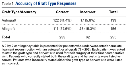
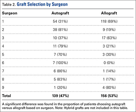
When asked which type of graft was used for their surgery, 12 of 304 patients (4%) did not know their graft type or harvest location. Twenty-nine patients stated that their graft was an allograft but did not know the harvest location. Five patients stated that their graft was an autograft but did not know the harvest location. The 34 patients who classified their choice of graft but did not know the harvest site (11%) stated their surgeon never told them where their graft was from or they did not remember. A complete list of graft type responses is shown in Table 3.
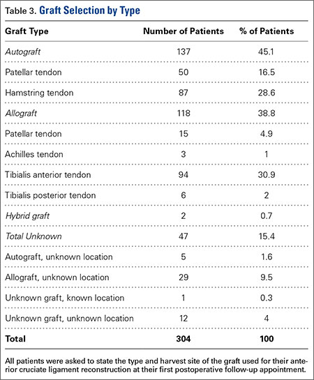
Of the 29 patients who stated that their graft was an allograft but did not know the harvest location, 19 (66%) had a tibialis anterior allograft, 7 (24%) had a BPTB allograft, 2 (7%) had an Achilles tendon allograft, and 1 (3%) had a tibialis anterior autograft.
Physician recommendation was the most important decision-making factor listed for 82% of patients at their first postoperative appointment (Table 4). In addition to the 4 factors listed on our survey, patients were allowed to write in other factors involved in their decision. The most popular answers included recovery time, personal research on graft types, and prior personal experience with ACL reconstruction on the contralateral knee.
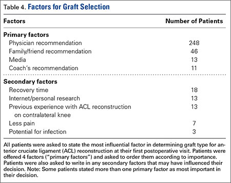
At the time of 1-year follow-up, 205 of 213 patients (96%) said they were satisfied with their graft choice (Table 5). All 4 unsatisfied autograft patients received a hamstring autograft, 3 of which were performed by the same surgeon. No significant difference was found in satisfaction rates between patients with autograft vs allograft (P = .87). There was a higher satisfaction rate among patients with a BPTB autograft compared to those with a hamstring autograft (P = .043). Of the unsatisfied patients, 3 patients stated that their graft had failed in the time prior to follow-up and 2 patients stated that they were having donor site pain following surgery with hamstring autograft and would consider an allograft if the reconstruction were repeated (Table 6). Two patients stated that they were unsatisfied with their graft but would need to do more research before deciding on a different graft type.
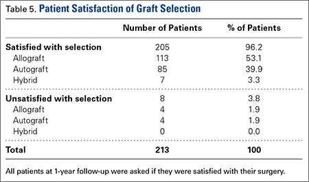
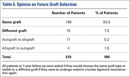
As shown in Tables 5 and 6, there is a discrepancy between the number of patients who were unsatisfied with their graft and the number of patients who stated that they would switch to a different graft type if they were to have ACL reconstruction again. A number of patients stated that they were satisfied with their graft, yet they would switch to a different graft. The main reasons for this related to issues from a hamstring autograft harvest site. One patient noted that although she was satisfied with her graft, she would switch after doing further research.
Discussion
Determining the decision-making factors for patients choosing between graft types for ACL reconstruction is important to ensure that patients can make a decision based on objective information. Several previous studies have evaluated patient selection of ACL grafts.8-10 All 3 of these studies showed that surgeon recommendation is the primary factor in a patient’s decision. Similar to previous studies, we also found that physician recommendation is the most influential factor involved in this decision.
At an average follow-up of 41 months, Cohen and colleagues8 found that 1.3% of patients did not know whether they received an autograft or allograft for their ACL reconstruction. Furthermore, 50.7% of patients stating they received an allograft in Cohen’s study8 were unsure of the harvest location. In our study, 4% of patients at their first postoperative visit did not know whether they had received an autograft or allograft and 10% of patients stating they received an allograft selected an unknown harvest site. In contrast, only 2% of autograft patients in our study were unsure of the harvest location at their first postoperative appointment. It is likely that, over time, patients with an allograft forget the harvest location, whereas autograft patients are more likely to remember the location of harvest. This is especially true in patients with anterior knee pain or hamstring pain following ACL reconstruction with a BPTB or hamstring tendon autograft, respectively.
In terms of patients’ knowledge of their graft type, we found an overall accuracy of 77%, with 88% of autograft patients, 71% of allograft patients, and 11% of hybrid graft patients remembering their graft type and harvest location. Although we do not believe it to be critical for patients to remember these details, we do believe that patients who do not know their graft type likely relied on the recommendation of their physician.
We found a significant difference in the proportion of patients choosing autograft vs allograft based on surgeon, despite these surgeons citing available data in the literature to each patient and ultimately allowing each patient to make his or her own decision. This is partly due to the low sample size of most of the surgeons involved. However, the main reason for this distortion is likely that different surgeons may highlight different aspects of the literature to “spin” patients towards one graft or another in certain cases.
Currently, there remains a lack of clarity in the literature on appropriate ACL graft choices for patients. With constant new findings being published on different aspects of various grafts, it is important for surgeons to remain up to date with the literature. Nevertheless, we believe that certain biases are inevitable among surgeons due to unique training experiences as well as experience with their own patients.
Cohen and colleagues8 found that only 7% of patients reported that their own personal research influenced their decision, and only 6.4% of patients reported the media as their primary decision-making factor. Cheung and colleagues9 conducted a retrospective study and found that more than half of patients did significant personal research prior to making a decision regarding their graft type. Most of this research was done using medical websites and literature. Koh and colleagues10 noted that >80% of patients consulted the internet for graft information before making a decision. Koh’s study10 was performed in Korea and therefore the high prevalence of internet use may be culturally-related.
Overall, quality of information for patients undergoing ACL reconstruction is mixed across the internet, with only 22.5% of top websites being affiliated with an academic institution and 35.5% of websites authored by private physicians or physician groups.11 Although a majority of internet websites offer discussion into the condition and surgical procedure of ACL reconstruction, less than half of these websites share the equally important information on the eligibility for surgery and concomitant complications following surgery.11In our study, only 39 patients (13%) listed the media as either the first (13, 4%) or second (26, 9%) most important factor in their graft decision. Clearly there is some discrepancy between studies regarding the influence of personal research and media. There are a few potential reasons for this. First, we did not explicitly ask patients if their own personal research had any influence on their graft decision. Rather, we asked patients to rank their decision-making factors, and few patients ranked the media as their first or second greatest influence. Second, the word “media” was used in our questionnaire rather than “online research” or “internet.” It may seem somewhat vague to patients what the word “media” really means in terms of their own research, whereas listing “online research” or “internet” as selection options may have influenced patient responses.
In our study, we asked patients for any additional factors that influenced their graft choice. Thirteen patients (4%) noted that “personal research” through internet, orthopaedic literature, and the media influenced their graft decision. This corroborates the idea that “media” may have seemed vague to some patients. Of these patients, 9 chose an autograft and 4 chose an allograft. The relative ease in accessing information regarding graft choice in ACL reconstruction should be noted. Numerous websites offer advice, graft options, and commentary from group practices and orthopaedic surgeons. Whether or not these sources provide reasonable support for one graft vs another graft remains to be answered. The physician should be responsible for providing the patient with this collected objective information.
In our study, 205 patients (96%) were satisfied with their graft choice at the time of follow-up, with 15 patients (7%) stating that they would have chosen a different graft type if they could redo the operation. Cheung and colleagues9 found a satisfaction rate of 87.4% at an average follow-up time of 19 months, with 4.6% stating they would have chosen a different graft type. Many factors can contribute to patient satisfaction after ACL reconstruction. Looking at patient variables such as age, demographics, occupation, activity level, surgical technique including tunnel placement and fixation, postoperative rehabilitation, and graft type may influence the success of the patient after ACL reconstruction.
The strengths of this study include the patient population size with 1-year follow-up as well as the prospective study design. In comparison to a previous retrospective study in 2009 by Cohen and colleagues8with a sample size of 240 patients, our study collected 213 patients with 70% follow-up at minimum 1 year. Collecting data prospectively ensures accurate representation of the factors influencing each patient’s graft selection, while follow-up data was useful for patient satisfaction.
The limitations of this study include the percentage of patients lost from follow-up as well as any bias generated from the organization of the questionnaire. Unfortunately, with a younger, transient population of patients undergoing ACL reconstruction in a major metropolitan area, a percentage of patients are lost to follow-up. Many attempts were made to locate these patients. Another potential limitation was the order of decision factors listed on the questionnaire. These factors were not ordered randomly on each survey, but were listed in the following order: (1) physician recommendation (2) family/friend’s recommendation (3) coach’s recommendation and (4) the media. This may have influenced patient responses. The organization of these factors in the questionnaire started with physician recommendation, which may have influenced the patient’s initial thought process of which factor had the greatest influence in their graft decision. In addition, for the surveys completed at least 1 year following surgery, some patients were contacted via e-mail and others via telephone. Thus, some patients may have changed their answers if they were able to see the questions rather than hearing the questions. We believe this is particularly true of the question regarding graft harvest site.
Our study indicates that the majority of patients undergoing ACL reconstruction are primarily influenced by the physician’s recommendation.
1. Madick S. Anterior cruciate ligament reconstruction of the knee. AORN J. 2011;93(2):210-222.
2. Baer GS, Harner CD. Clinical outcomes of allograft versus autograft in anterior cruciate ligament reconstruction. Clin Sports Med. 2007;26(4):661-681.
3. Paxton EW, Namba RS, Maletis GB, et al. A prospective study of 80,000 total joint and 5000 anterior cruciate ligament reconstruction procedures in a community-based registry in the United States. J Bone Joint Surg Am. 2010;92(suppl 2):117-132.
4. Kraeutler MJ, Bravman JT, McCarty EC. Bone-patellar tendon-bone autograft versus allograft in outcomes of anterior cruciate ligament reconstruction: A meta-analysis of 5182 patients. Am J Sports Med. 2013;41(10):2439-2448.
5. Spindler KP, Kuhn JE, Freedman KB, Matthews CE, Dittus RS, Harrell FE Jr. Anterior cruciate ligament reconstruction autograft choice: bone-tendon-bone versus hamstring: does it really matter? A systematic review. Am J Sports Med. 2004;32(8):1986-1995.
6. Boonriong T, Kietsiriroje N. Arthroscopically assisted anterior cruciate ligament reconstruction: comparison of bone-patellar tendon-bone versus hamstring tendon autograft. J Med Assoc Thai. 2004;87(9):1100-1107.
7. Fox JA, Pierce M, Bojchuk J, Hayden J, Bush-Joseph CA, Bach BR Jr. Revision anterior cruciate ligament reconstruction with nonirradiated fresh-frozen patellar tendon allograft. Arthroscopy. 2004;20(8):787-794.
8. Cohen SB, Yucha DT, Ciccotti MC, Goldstein DT, Ciccotti MA, Ciccotti MG. Factors affecting patient selection of graft type in anterior cruciate ligament reconstruction. Arthroscopy. 2009;25(9):1006-1010.
9. Cheung SC, Allen CR, Gallo RA, Ma CB, Feeley BT. Patients’ attitudes and factors in their selection of grafts for anterior cruciate ligament reconstruction. Knee. 2012;19(1):49-54.
10. Koh HS, In Y, Kong CG, Won HY, Kim KH, Lee JH. Factors affecting patients’ graft choice in anterior cruciate ligament reconstruction. Clin Orthop Surg. 2010;2(2):69-75.
11. Duncan IC, Kane PW, Lawson KA, Cohen SB, Ciccotti MG, Dodson CC. Evaluation of information available on the internet regarding anterior cruciate ligament reconstruction. Arthroscopy. 2013;29(6):1101-1107.
Anterior cruciate ligament (ACL) injuries affect >175,000 people each year,1 with >100,000 Americans undergoing ACL reconstruction annually.2 Due to the high impact this injury has on the general population, and especially on athletes, it is important to determine the factors that influence a patient’s selection of a particular graft type. With increasing access to information and other outside influences, surgeons should attempt to provide as much objective information as possible in order to allow patients to make appropriate informed decisions regarding their graft choice for ACL surgery.
While autografts are used in >60% of primary ACL reconstructions, allografts are used in >80% of revision procedures.3 Both autografts and allografts offer advantages and disadvantages, and the advantages of each may depend on patient age, activity level, and occupation.4 For example, graft rerupture rates have been shown to be higher in patients with ACL allografts4, while kneeling pain has been shown to be worse in patients with bone-patellar tendon-bone (BPTB) autografts compared to hamstring autografts5 as well as BPTB allografts.4
Patient satisfaction rates are high for ACL autografts and allografts. Boonriong and Kietsiriroje6 have shown visual analog scale (VAS) patient satisfaction score averages to be 88 out of 100 for BPTB autografts and 93 out of 100 for hamstring tendon autografts. Fox and colleagues7 showed that 87% of patients were completely or mostly satisfied following revision ACL reconstruction with patellar tendon allograft. Cohen and colleagues8 evaluated 240 patients undergoing primary ACL reconstruction; 63.3% underwent ACL reconstruction with an allograft and 35.4% with an autograft. Of all patients enrolled in the study, 93% were satisfied with their graft choice, with 12.7% of patients opting to choose another graft if in the same situation again. Of those patients, 63.3% would have switched from an autograft to allograft. Although these numbers represent high patient satisfaction following a variety of ACL graft types, it is important to continue to identify graft selection factors in order to maximize patient outcomes.
The purposes of this prospective study were to assess patients’ knowledge of their graft type used for ACL reconstruction, to determine the most influential factors involved in graft selection, and to determine the level of satisfaction with the graft of choice at a minimum of 1-year follow-up. Based on a previous retrospective study,8 we hypothesized that physician recommendation would be the most influential factor in ACL graft selection. We also hypothesized that patients receiving an autograft would be more accurate in stating their graft harvest location compared to allograft patients.
Materials and Methods
We prospectively enrolled 304 patients who underwent primary ACL reconstruction from January 2008 to September 2013. Surgery was performed by 9 different surgeons within the same practice. All patients undergoing primary ACL reconstruction were eligible for the study.
All surgeons explained to each patient the pros and cons of each graft choice based upon peer-reviewed literature. Each patient was allowed to choose autograft or allograft, although most of the surgeons strongly encourage patients under age 25 years to choose autograft. One of the surgeons specifically encourages a patellar tendon autograft in patients under age 30 to 35 years, except for those patients with a narrow patellar tendon on magnetic resonance imaging, in which case he recommends a hamstring autograft. Another surgeon also specifically encourages patellar tendon autograft in patients under 35 years, except in skeletally immature patients, for whom he encourages hamstring autograft. However, none of the surgeons prohibited patients from choosing autograft or allograft, regardless of age.
The Institutional Review Board at our institution provided approval for this study. At the first postoperative follow-up appointment, each patient completed a questionnaire asking to select from a list the type (“your own” or “a cadaver”) and harvest site of the graft that was used for the surgery. Patients were also asked how they decided upon that graft type by ranking a list of 4 factors from 1 to 4. These included (1) physician recommendation, (2) family/friend’s recommendation, (3) coach’s recommendation, and (4) the media. Patients had the option of ranking more than one factor as most important in their decision. In addition, patients were asked to list any other factors that influenced their decision regarding graft type.
At a minimum of 1 year following surgery, patients completed the same questionnaire described above. In addition, patients were asked if they were satisfied with their graft and whether they would choose the same graft type if undergoing ACL reconstruction again. Patients who would have chosen a different graft were asked which graft they would have chosen and why. Any patient who experienced graft rupture prior to follow-up was included in the analysis.
Statistical Analysis
Chi square tests were used to compare dichotomous outcomes. A type I error of less than 5% (P < .05) was considered statistically significant.
Results
At least 1 year following ACL reconstruction, 213 of 304 patients (70%) successfully completed the same questionnaire as they did at their first postoperative follow-up appointment. The mean age of these patients at the time of surgery was 31.9 ± 11.0 years (range, 13.9 to 58.0 years). The mean follow-up time was 1.4 ± 0.4 years (range, 1.0 to 2.6 years), and 59% of these patients were male.
Autografts were used for 139 patients (139/304, 46%), allografts for 156 patients (156/304, 51%), and hybrid grafts for 9 patients (9/304, 3%). Overall, 77% of patients were accurate in stating the type of graft used for their ACL reconstruction, including 88% of autograft patients, 71% of allograft patients, and 11% of hybrid graft patients (Table 1). Patients who underwent reconstruction with an autograft were significantly more accurate in stating their graft type compared to patients with an allograft (P < .001). Graft type by surgeon is shown in Table 2. A statistically significant difference was found in the proportion of patients choosing autograft versus allograft based on surgeon (P < .0001).
When asked which type of graft was used for their surgery, 12 of 304 patients (4%) did not know their graft type or harvest location. Twenty-nine patients stated that their graft was an allograft but did not know the harvest location. Five patients stated that their graft was an autograft but did not know the harvest location. The 34 patients who classified their choice of graft but did not know the harvest site (11%) stated their surgeon never told them where their graft was from or they did not remember. A complete list of graft type responses is shown in Table 3.
Of the 29 patients who stated that their graft was an allograft but did not know the harvest location, 19 (66%) had a tibialis anterior allograft, 7 (24%) had a BPTB allograft, 2 (7%) had an Achilles tendon allograft, and 1 (3%) had a tibialis anterior autograft.
Physician recommendation was the most important decision-making factor listed for 82% of patients at their first postoperative appointment (Table 4). In addition to the 4 factors listed on our survey, patients were allowed to write in other factors involved in their decision. The most popular answers included recovery time, personal research on graft types, and prior personal experience with ACL reconstruction on the contralateral knee.
At the time of 1-year follow-up, 205 of 213 patients (96%) said they were satisfied with their graft choice (Table 5). All 4 unsatisfied autograft patients received a hamstring autograft, 3 of which were performed by the same surgeon. No significant difference was found in satisfaction rates between patients with autograft vs allograft (P = .87). There was a higher satisfaction rate among patients with a BPTB autograft compared to those with a hamstring autograft (P = .043). Of the unsatisfied patients, 3 patients stated that their graft had failed in the time prior to follow-up and 2 patients stated that they were having donor site pain following surgery with hamstring autograft and would consider an allograft if the reconstruction were repeated (Table 6). Two patients stated that they were unsatisfied with their graft but would need to do more research before deciding on a different graft type.
As shown in Tables 5 and 6, there is a discrepancy between the number of patients who were unsatisfied with their graft and the number of patients who stated that they would switch to a different graft type if they were to have ACL reconstruction again. A number of patients stated that they were satisfied with their graft, yet they would switch to a different graft. The main reasons for this related to issues from a hamstring autograft harvest site. One patient noted that although she was satisfied with her graft, she would switch after doing further research.
Discussion
Determining the decision-making factors for patients choosing between graft types for ACL reconstruction is important to ensure that patients can make a decision based on objective information. Several previous studies have evaluated patient selection of ACL grafts.8-10 All 3 of these studies showed that surgeon recommendation is the primary factor in a patient’s decision. Similar to previous studies, we also found that physician recommendation is the most influential factor involved in this decision.
At an average follow-up of 41 months, Cohen and colleagues8 found that 1.3% of patients did not know whether they received an autograft or allograft for their ACL reconstruction. Furthermore, 50.7% of patients stating they received an allograft in Cohen’s study8 were unsure of the harvest location. In our study, 4% of patients at their first postoperative visit did not know whether they had received an autograft or allograft and 10% of patients stating they received an allograft selected an unknown harvest site. In contrast, only 2% of autograft patients in our study were unsure of the harvest location at their first postoperative appointment. It is likely that, over time, patients with an allograft forget the harvest location, whereas autograft patients are more likely to remember the location of harvest. This is especially true in patients with anterior knee pain or hamstring pain following ACL reconstruction with a BPTB or hamstring tendon autograft, respectively.
In terms of patients’ knowledge of their graft type, we found an overall accuracy of 77%, with 88% of autograft patients, 71% of allograft patients, and 11% of hybrid graft patients remembering their graft type and harvest location. Although we do not believe it to be critical for patients to remember these details, we do believe that patients who do not know their graft type likely relied on the recommendation of their physician.
We found a significant difference in the proportion of patients choosing autograft vs allograft based on surgeon, despite these surgeons citing available data in the literature to each patient and ultimately allowing each patient to make his or her own decision. This is partly due to the low sample size of most of the surgeons involved. However, the main reason for this distortion is likely that different surgeons may highlight different aspects of the literature to “spin” patients towards one graft or another in certain cases.
Currently, there remains a lack of clarity in the literature on appropriate ACL graft choices for patients. With constant new findings being published on different aspects of various grafts, it is important for surgeons to remain up to date with the literature. Nevertheless, we believe that certain biases are inevitable among surgeons due to unique training experiences as well as experience with their own patients.
Cohen and colleagues8 found that only 7% of patients reported that their own personal research influenced their decision, and only 6.4% of patients reported the media as their primary decision-making factor. Cheung and colleagues9 conducted a retrospective study and found that more than half of patients did significant personal research prior to making a decision regarding their graft type. Most of this research was done using medical websites and literature. Koh and colleagues10 noted that >80% of patients consulted the internet for graft information before making a decision. Koh’s study10 was performed in Korea and therefore the high prevalence of internet use may be culturally-related.
Overall, quality of information for patients undergoing ACL reconstruction is mixed across the internet, with only 22.5% of top websites being affiliated with an academic institution and 35.5% of websites authored by private physicians or physician groups.11 Although a majority of internet websites offer discussion into the condition and surgical procedure of ACL reconstruction, less than half of these websites share the equally important information on the eligibility for surgery and concomitant complications following surgery.11In our study, only 39 patients (13%) listed the media as either the first (13, 4%) or second (26, 9%) most important factor in their graft decision. Clearly there is some discrepancy between studies regarding the influence of personal research and media. There are a few potential reasons for this. First, we did not explicitly ask patients if their own personal research had any influence on their graft decision. Rather, we asked patients to rank their decision-making factors, and few patients ranked the media as their first or second greatest influence. Second, the word “media” was used in our questionnaire rather than “online research” or “internet.” It may seem somewhat vague to patients what the word “media” really means in terms of their own research, whereas listing “online research” or “internet” as selection options may have influenced patient responses.
In our study, we asked patients for any additional factors that influenced their graft choice. Thirteen patients (4%) noted that “personal research” through internet, orthopaedic literature, and the media influenced their graft decision. This corroborates the idea that “media” may have seemed vague to some patients. Of these patients, 9 chose an autograft and 4 chose an allograft. The relative ease in accessing information regarding graft choice in ACL reconstruction should be noted. Numerous websites offer advice, graft options, and commentary from group practices and orthopaedic surgeons. Whether or not these sources provide reasonable support for one graft vs another graft remains to be answered. The physician should be responsible for providing the patient with this collected objective information.
In our study, 205 patients (96%) were satisfied with their graft choice at the time of follow-up, with 15 patients (7%) stating that they would have chosen a different graft type if they could redo the operation. Cheung and colleagues9 found a satisfaction rate of 87.4% at an average follow-up time of 19 months, with 4.6% stating they would have chosen a different graft type. Many factors can contribute to patient satisfaction after ACL reconstruction. Looking at patient variables such as age, demographics, occupation, activity level, surgical technique including tunnel placement and fixation, postoperative rehabilitation, and graft type may influence the success of the patient after ACL reconstruction.
The strengths of this study include the patient population size with 1-year follow-up as well as the prospective study design. In comparison to a previous retrospective study in 2009 by Cohen and colleagues8with a sample size of 240 patients, our study collected 213 patients with 70% follow-up at minimum 1 year. Collecting data prospectively ensures accurate representation of the factors influencing each patient’s graft selection, while follow-up data was useful for patient satisfaction.
The limitations of this study include the percentage of patients lost from follow-up as well as any bias generated from the organization of the questionnaire. Unfortunately, with a younger, transient population of patients undergoing ACL reconstruction in a major metropolitan area, a percentage of patients are lost to follow-up. Many attempts were made to locate these patients. Another potential limitation was the order of decision factors listed on the questionnaire. These factors were not ordered randomly on each survey, but were listed in the following order: (1) physician recommendation (2) family/friend’s recommendation (3) coach’s recommendation and (4) the media. This may have influenced patient responses. The organization of these factors in the questionnaire started with physician recommendation, which may have influenced the patient’s initial thought process of which factor had the greatest influence in their graft decision. In addition, for the surveys completed at least 1 year following surgery, some patients were contacted via e-mail and others via telephone. Thus, some patients may have changed their answers if they were able to see the questions rather than hearing the questions. We believe this is particularly true of the question regarding graft harvest site.
Our study indicates that the majority of patients undergoing ACL reconstruction are primarily influenced by the physician’s recommendation.
1. Madick S. Anterior cruciate ligament reconstruction of the knee. AORN J. 2011;93(2):210-222.
2. Baer GS, Harner CD. Clinical outcomes of allograft versus autograft in anterior cruciate ligament reconstruction. Clin Sports Med. 2007;26(4):661-681.
3. Paxton EW, Namba RS, Maletis GB, et al. A prospective study of 80,000 total joint and 5000 anterior cruciate ligament reconstruction procedures in a community-based registry in the United States. J Bone Joint Surg Am. 2010;92(suppl 2):117-132.
4. Kraeutler MJ, Bravman JT, McCarty EC. Bone-patellar tendon-bone autograft versus allograft in outcomes of anterior cruciate ligament reconstruction: A meta-analysis of 5182 patients. Am J Sports Med. 2013;41(10):2439-2448.
5. Spindler KP, Kuhn JE, Freedman KB, Matthews CE, Dittus RS, Harrell FE Jr. Anterior cruciate ligament reconstruction autograft choice: bone-tendon-bone versus hamstring: does it really matter? A systematic review. Am J Sports Med. 2004;32(8):1986-1995.
6. Boonriong T, Kietsiriroje N. Arthroscopically assisted anterior cruciate ligament reconstruction: comparison of bone-patellar tendon-bone versus hamstring tendon autograft. J Med Assoc Thai. 2004;87(9):1100-1107.
7. Fox JA, Pierce M, Bojchuk J, Hayden J, Bush-Joseph CA, Bach BR Jr. Revision anterior cruciate ligament reconstruction with nonirradiated fresh-frozen patellar tendon allograft. Arthroscopy. 2004;20(8):787-794.
8. Cohen SB, Yucha DT, Ciccotti MC, Goldstein DT, Ciccotti MA, Ciccotti MG. Factors affecting patient selection of graft type in anterior cruciate ligament reconstruction. Arthroscopy. 2009;25(9):1006-1010.
9. Cheung SC, Allen CR, Gallo RA, Ma CB, Feeley BT. Patients’ attitudes and factors in their selection of grafts for anterior cruciate ligament reconstruction. Knee. 2012;19(1):49-54.
10. Koh HS, In Y, Kong CG, Won HY, Kim KH, Lee JH. Factors affecting patients’ graft choice in anterior cruciate ligament reconstruction. Clin Orthop Surg. 2010;2(2):69-75.
11. Duncan IC, Kane PW, Lawson KA, Cohen SB, Ciccotti MG, Dodson CC. Evaluation of information available on the internet regarding anterior cruciate ligament reconstruction. Arthroscopy. 2013;29(6):1101-1107.
Actinic Keratosis as a Marker of Field Cancerization in Excision Specimens of Cutaneous Malignancies
The concept of field cancerization was first proposed in 1953 by Slaughter et al1 in their study of oral squamous carcinomas. Their findings of multifocal patches of premalignant disease, abnormal tissue surrounding tumors, multiple localized primary tumors, and tumor recurrence following surgical resection was suggestive of a field of dysplastic cells with malignant potential.1 Since then, modern molecular techniques have been used to establish a genetic basis for this model in many different types of cancer, including cutaneous malignancies.2-4 The field begins from a singular stem cell, which undergoes one or more genetic changes that allow for a growth advantage compared to surrounding cells. The stem cell then divides, forming a patch of clonal daughter cells that displace the surrounding normal epithelium. Growth of this patch eventually leads to a dysplastic field of monoclonal cells, which notably does not yet show invasive growth or metastatic behavior. Over time, continued carcinogenic exposure results in additional genetic alterations among different cells in the field, which leads to new subclonal proliferations that share common clonal origin but exhibit unique genetic changes. Eventually, transformative events may occur, resulting in cells with invasive and metastatic properties, thus forming a carcinoma.5
In the case of cutaneous malignancies, UV radiation in the form of UVA and UVB rays is the most common source of carcinogenesis. It is well established that UV radiation has numerous effects on the body, including but not limited to local and systemic immunosuppression, alteration of signal transduction pathways, and the development of mutations in DNA via direct damage by UVB or indirect damage by free radical formation with UVA.6,7 Normally, DNA is protected from UV radiation–induced genetic alteration by the p53 gene, TP53. As such, damage to this gene is highly associated with cancer induction. One study found that more than 90% of squamous cell carcinomas (SCCs) and more than 50% of basal cell carcinomas (BCCs) contain UV-like mutations in TP53.8 The concept of field cancerization suggests that because the skin surrounding cutaneous malignancies has been exposed to the same chronic UV light as the initial lesion, it is at an increased risk for genetic abnormalities and thus possible malignant transformation.
Actinic keratoses (AKs) are common neoplasms of the skin that generally are regarded as precancerous lesions or may be considered to be the earliest stage of SCC in situ.9 Actinic keratoses usually develop as a consequence of chronic exposure to UV radiation and often are clinically apparent as erythematous scaly papules in sun-exposed areas (Figure 1).10 They also are identified histologically as atypical keratinocytes along the basal layer of the epidermis with possible enlargement, hyperchromatic nuclei, lack of maturation, mitotic figures, inflammatory infiltrate, and/or hyperkeratosis.10 Furthermore, the genetic changes associated with AKs are well documented and are strongly associated with changes to p53.11 Given these characteristics, AKs serve as good markers of genetic damage with potential for malignancy. In this study, we used histologically identified AKs to assess the presence of field damage in the tissue immediately surrounding excision specimens of SCCs, BCCs, and malignant melanomas (MMs).
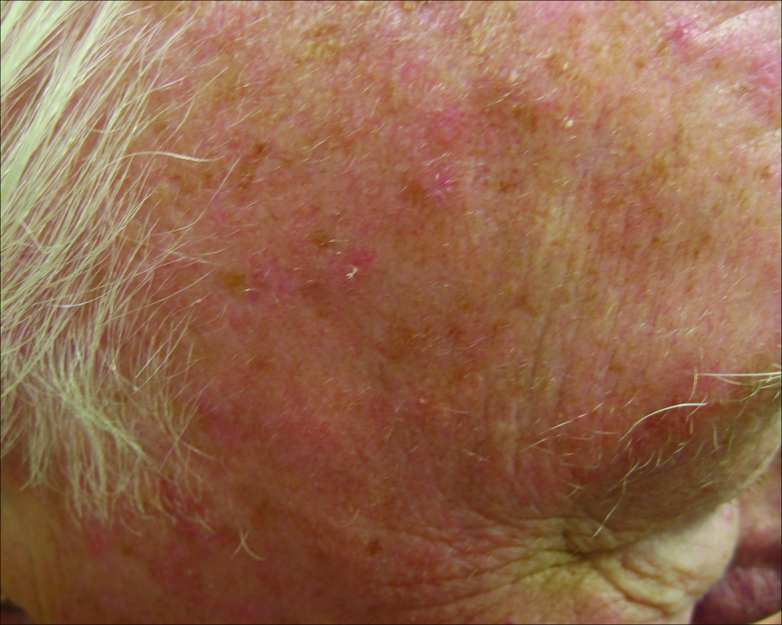
Methods
This study was approved by the Program for the Protection of Human Subjects at the Icahn School of Medicine at Mount Sinai (New York, New York) prior to initiation. All cutaneous specimens submitted to the dermatopathology service for consultation between April 2013 and June 2013 were reviewed for inclusion in this study. Data collection was extended for MMs to include all specimens from January 2013 to June 2013 given the limited number of cases in the original data collection period.
Initial screening for this study was done electronically and assessed for a diagnosis of SCC (Figure 2), BCC (Figure 3), or MM (Figure 4) as determined by a board-certified dermatopathologist (G.G.). The resulting pool of specimens was then screened to include only excision specimens and to exclude curettage specimens and superficial specimens that lacked dermis. In this study, we chose to look at reexcisions rather than initial biopsies so that there was a greater likelihood of having an intact epidermis surrounding a malignancy that could be assessed for the presence of AKs as markers for field cancerization. Specimens were examined in full via serial transverse cross-sections at 3-mm intervals. Additional step sections were obtained at smaller intervals when margins were close or unclear.
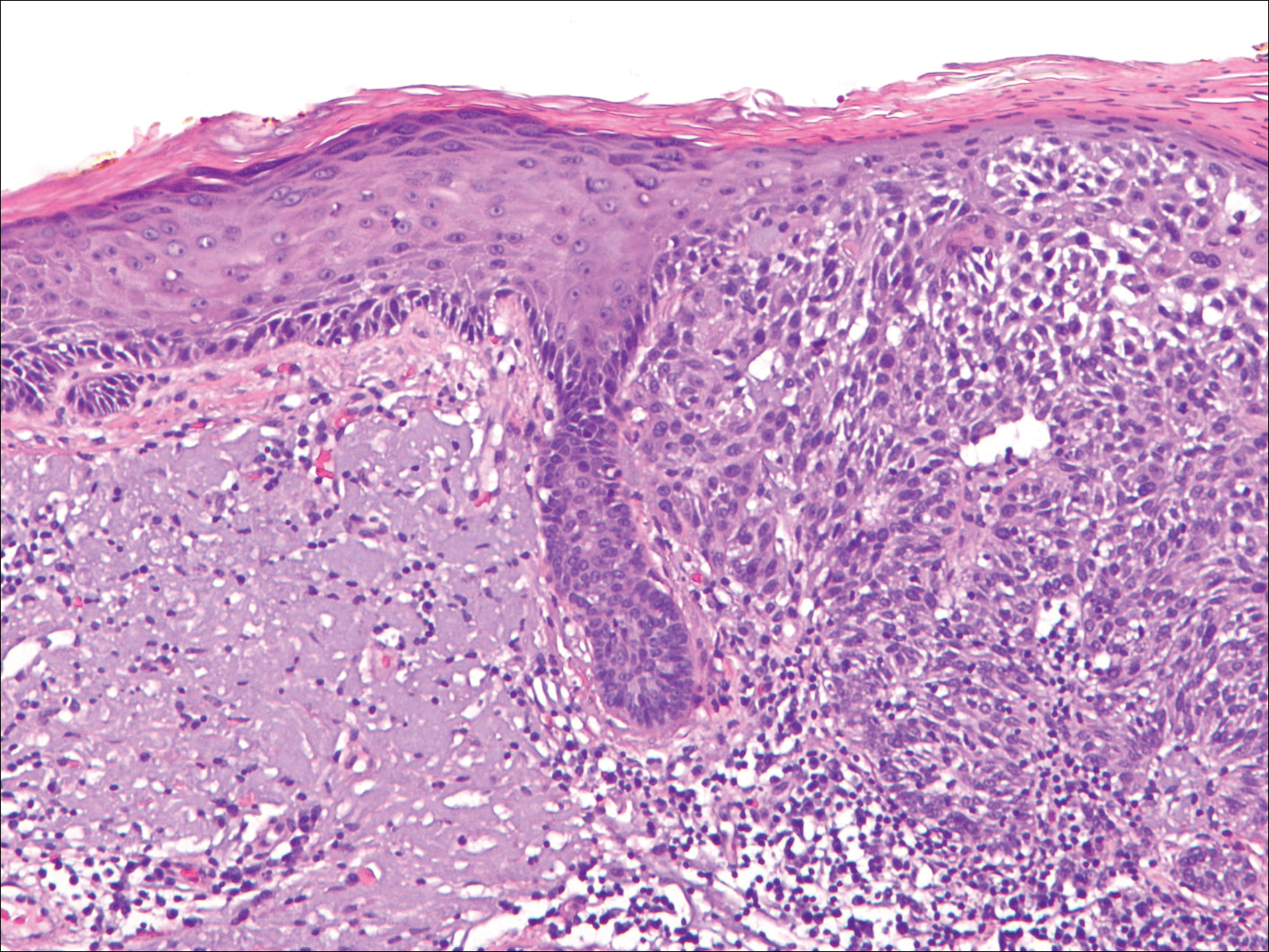
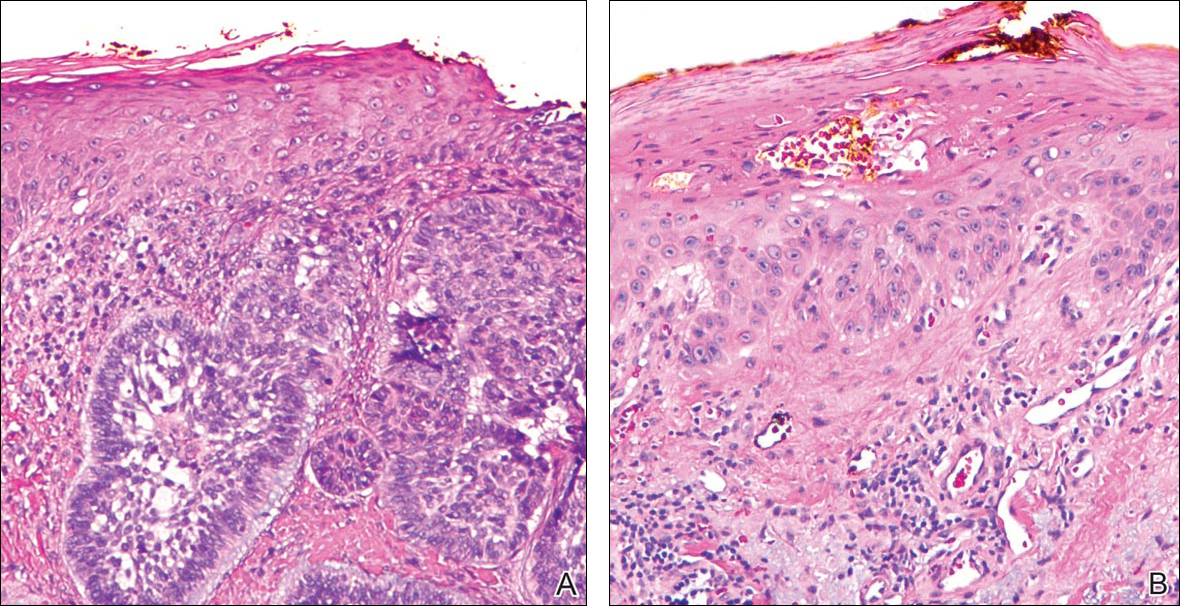
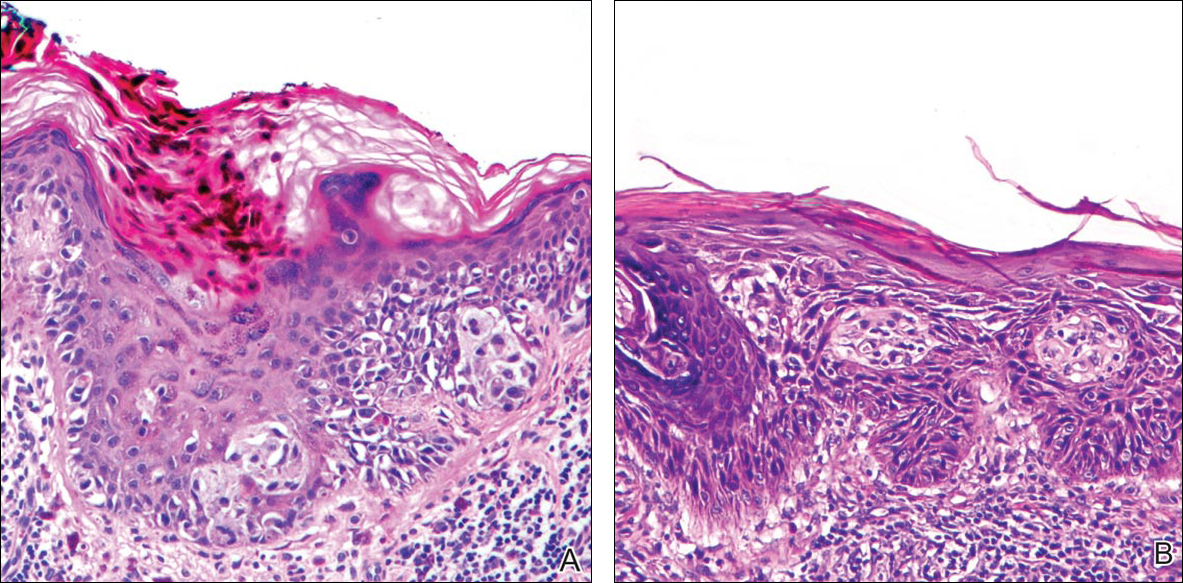
Selected cases were reassessed by a board-certified dermatopathologist (G.G.) to confirm the diagnosis and to assess for the presence of at least 1 AK within the specimen sample that was separated from the original malignancy by histologically normal-appearing cells. Samples were also assessed for the presence of an AK within 0.1 mm of the distal lateral margins of the tissue sample. Information regarding patient age, gender, lesion location, lesion type, and specimen size was collected for each sample. In accordance with institutional review board protocol, research data were collected without any protected health information. All analyses and results were deidentified and stored on a password-protected computer database. Statistical analysis was performed using SPSS software. When applicable, P<.05 was considered to indicate statistical significance.
Results
There were 205 cases that passed the initial screening filters, of which 56 were excluded due to the presence of curettage or lack of a sufficient tissue sample. Of the remaining 149 cases, the distribution by malignancy type was tabulated along with the percentage of observed AKs. If an AK was observed, the percentage that had an AK at the lateral margins (marginal AK) was determined (Table 1). A χ2 analysis determined that AKs were observed significantly more often in SCC specimens (57% [35/61]) than BCC (33% [21/64]) or malignant melanoma (25% [6/24]) specimens (P=.0125).
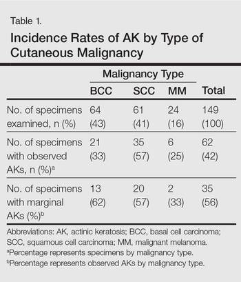
Statistics regarding patient age and gender as well as specimen size were stratified by malignancy type (Table 2). Using a receiver operating characteristic curve and the Youden index, an optimal cutoff of older than 67 years was determined to increase probability of observing an AK (P=.077) with sensitivity of 0.531 and specificity of 0.529. The distribution of specimen excision location for each malignancy type is shown in Table 3.
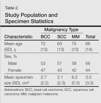
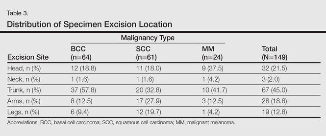
A multivariate analysis was performed to determine if the variables of patient age, gender, biopsy size, malignancy type (SCC, BCC, or MM), or cancer location (head, neck, trunk, arms, or legs) were independently useful in predicting whether an AK would be observed in the excision specimen. The significance of variables in the logistic regression model was assessed using a backward stepwise regression selection procedure entering variables if P<.15 and excluding variables if P>.25. Significant variables in predicting the occurrence of AK were SCC malignancy type (P=.007; odds ratio [OR], 2.61) and location on the head (P=.044; OR, 2.39) and arms (P=.042; OR, 2.55).
Comment
The χ2 analysis of our data showed that SCC specimens were significantly more likely to have an associated AK than either BCCs or MMs (P=.0125), which is not surprising given that AKs are considered by many to be early-stage SCCs.12 It is important to note, however, that BCCs and MMs both had nonnegligible rates of associated AKs. Although BCC and MM do not arise from the same background of genetic changes as SCC, this finding is noteworthy because it demonstrates definitive field damage with malignant potential in the area surrounding these cutaneous malignancies.
Our data also showed that there was a significantly greater association of AKs in malignancies located on the head (P=.044) and arms (P=.042), possibly because these 2 areas tend to be the most sun exposed and thus are more likely to have sustained field damage as evidenced by the higher percentage of AKs. A study by Jonason et al13 described a similar finding in which sun-exposed skin exhibited significantly more frequent (P=.04) and larger (P=.02) clonal patches of mutated p53 keratinocytes than sun-protected skin.
It is likely that the field damage surrounding the cutaneous lesions in our study is actually greater than what we reported because the AK was present at the margin of the excision specimens the majority of the time (56%), which suggests that there likely may have been more AKs found if a wider area surrounding the malignancy had been studied given that AKs often are at the periphery of the lesion and may be missed by a small excision. Fewer marginal AKs were observed with MM cases, possibly because the excision specimens were more than double the size of SCC or BCC excisions. Furthermore, there likely is to be more damage than what can be appreciated by visual changes alone.
Kanjilal et al14 used polymerase chain reaction and DNA sequencing to demonstrate numerous p53 mutations in nonmalignant-appearing skin surrounding BCCs and SCCs. Brennan et al15 found p53 mutations in surgical margins of excised SCCs considered to be tumor free by histopathologic analysis in more than half of the specimens studied. Notably, tumor recurrence was significantly more likely in areas where mutations were found and no tumor recurrence was seen in areas free of p53 mutations (P=.02).15 Tabor et al4 similarly found genetically altered fields in histologically clear surgical margins of SCCs but also showed that local tumor recurrence following excision had more molecular markers in common with the nonresected premalignant field than it did with the primary tumor. Thus, these studies provide a genetic basis for field damage that can exist even in histologically benign-appearing cells.
We believe our findings are clinically relevant, as they provide additional evidence for the theory of field cancerization as demonstrated by the nonnegligible rates of AKs and thus field damage with malignant potential in the skin immediately surrounding cutaneous malignancies. The limitations of our study, however, include a small sample size; no consideration of the effects of prior topical, field, or systemic treatments; and lack of a control group. Nevertheless, our findings emphasize the importance of assessing the extent of field damage when determining treatment strategies. Clinicians treating cutaneous malignancies should consider the need for field therapy, especially in sun-exposed regions, to avoid additional primary tumors.16 Further research is needed, however, to identify optimal methods for quantifying field damage clinically and determining the most effective treatment strategies.
- Slaughter DP, Southwick HW, Smejkal W. Field cancerization in oral stratified squamous epithelium; clinical implications of multicentric origin. Cancer. 1953;6:963-968.
- Braakhuis B, Tabor M, Kummer J, et al. A genetic explanation of Slaughter’s concept of field cancerization: evidence and clinical implications. Cancer Res. 2003;63:1727-1730.
- Stern R, Bolshakov S, Nataraj A, et al. p53 Mutation in nonmelanoma skin cancers occurring in psoralen ultraviolet A-treated patients: evidence for heterogeneity and field cancerization. J Invest Dermatol. 2002;119:522-526.
- Tabor M, Brakenhoff R, van Houten VM, et al. Persistence of genetically altered fields in head and neck cancer patients: biological and clinical implications. Clin Cancer Res. 2001;7:1523-1532.
- Torezan L. Cutaneous field cancerization: clinical, histopathological and therapeutic aspects. An Bras Dermatol. 2013;88:775-786.
- Ullrich S, Kripke M, Ananthaswamy H. Mechanisms underlying UV-induced immune suppression: implications for sunscreen design. Exp Dermatol. 2002;11:1-4.
- de Gruijl FR. Photocarcinogenesis: UVA vs UVB. Methods Enzymol. 2000;319:359-366.
- Brash DE, Ziegler A, Jonason AS, et al. Sunlight and sunburn in human skin cancer: p53, apoptosis, and tumor promotion. J Investig Dermatol Symp Proc. 1996;1:136-142.
- Ackerman AB, Mones JM. Solar (actinic) keratosis is squamous cell carcinoma. Br J Dermatol. 2006;155:9-22.
- Rossi R, Mori M, Lotti T. Actinic keratosis. Int J Dermatol. 2007;46:895-904.
- Ziegler A, Jonason AS, Leffel DJ, et al. Sunburn and p53 in the onset of skin cancer. Nature. 1994;372:773-776.
- Cockerell C. Histopathology of incipient intraepidermal squamous cell carcinoma (“actinic keratosis”). J Am Acad Dermatol. 2000;42:11-17.
- Jonason AS, Kunala S, Price GJ, et al. Frequent clones of p53-mutated keratinocytes in normal human skin. Proc Natl Acad Sci. 1996;93:14025-14029.
- Kanjilal S, Strom SS, Clayman GL, et al. p53 Mutations in nonmelanoma skin cancer of the head and neck: molecular evidence for field cancerization. Cancer Res. 1995;55:3604-3609.
- Brennan JA, Mao L, Hruban RH, et al. Molecular assessment of histopathological staging in squamous cell carcinoma of the head and neck. N Engl J Med. 1995;332:429-435.
- Braathen LR, Morton CA, Basset-Seguin N, et al. Photodynamic therapy for skin field cancerization: an international consensus. International Society for Photodynamic Therapy in Dermatology. J Eur Acad Dermatol Venereol. 2012;26:1063-1066.
The concept of field cancerization was first proposed in 1953 by Slaughter et al1 in their study of oral squamous carcinomas. Their findings of multifocal patches of premalignant disease, abnormal tissue surrounding tumors, multiple localized primary tumors, and tumor recurrence following surgical resection was suggestive of a field of dysplastic cells with malignant potential.1 Since then, modern molecular techniques have been used to establish a genetic basis for this model in many different types of cancer, including cutaneous malignancies.2-4 The field begins from a singular stem cell, which undergoes one or more genetic changes that allow for a growth advantage compared to surrounding cells. The stem cell then divides, forming a patch of clonal daughter cells that displace the surrounding normal epithelium. Growth of this patch eventually leads to a dysplastic field of monoclonal cells, which notably does not yet show invasive growth or metastatic behavior. Over time, continued carcinogenic exposure results in additional genetic alterations among different cells in the field, which leads to new subclonal proliferations that share common clonal origin but exhibit unique genetic changes. Eventually, transformative events may occur, resulting in cells with invasive and metastatic properties, thus forming a carcinoma.5
In the case of cutaneous malignancies, UV radiation in the form of UVA and UVB rays is the most common source of carcinogenesis. It is well established that UV radiation has numerous effects on the body, including but not limited to local and systemic immunosuppression, alteration of signal transduction pathways, and the development of mutations in DNA via direct damage by UVB or indirect damage by free radical formation with UVA.6,7 Normally, DNA is protected from UV radiation–induced genetic alteration by the p53 gene, TP53. As such, damage to this gene is highly associated with cancer induction. One study found that more than 90% of squamous cell carcinomas (SCCs) and more than 50% of basal cell carcinomas (BCCs) contain UV-like mutations in TP53.8 The concept of field cancerization suggests that because the skin surrounding cutaneous malignancies has been exposed to the same chronic UV light as the initial lesion, it is at an increased risk for genetic abnormalities and thus possible malignant transformation.
Actinic keratoses (AKs) are common neoplasms of the skin that generally are regarded as precancerous lesions or may be considered to be the earliest stage of SCC in situ.9 Actinic keratoses usually develop as a consequence of chronic exposure to UV radiation and often are clinically apparent as erythematous scaly papules in sun-exposed areas (Figure 1).10 They also are identified histologically as atypical keratinocytes along the basal layer of the epidermis with possible enlargement, hyperchromatic nuclei, lack of maturation, mitotic figures, inflammatory infiltrate, and/or hyperkeratosis.10 Furthermore, the genetic changes associated with AKs are well documented and are strongly associated with changes to p53.11 Given these characteristics, AKs serve as good markers of genetic damage with potential for malignancy. In this study, we used histologically identified AKs to assess the presence of field damage in the tissue immediately surrounding excision specimens of SCCs, BCCs, and malignant melanomas (MMs).
Methods
This study was approved by the Program for the Protection of Human Subjects at the Icahn School of Medicine at Mount Sinai (New York, New York) prior to initiation. All cutaneous specimens submitted to the dermatopathology service for consultation between April 2013 and June 2013 were reviewed for inclusion in this study. Data collection was extended for MMs to include all specimens from January 2013 to June 2013 given the limited number of cases in the original data collection period.
Initial screening for this study was done electronically and assessed for a diagnosis of SCC (Figure 2), BCC (Figure 3), or MM (Figure 4) as determined by a board-certified dermatopathologist (G.G.). The resulting pool of specimens was then screened to include only excision specimens and to exclude curettage specimens and superficial specimens that lacked dermis. In this study, we chose to look at reexcisions rather than initial biopsies so that there was a greater likelihood of having an intact epidermis surrounding a malignancy that could be assessed for the presence of AKs as markers for field cancerization. Specimens were examined in full via serial transverse cross-sections at 3-mm intervals. Additional step sections were obtained at smaller intervals when margins were close or unclear.
Selected cases were reassessed by a board-certified dermatopathologist (G.G.) to confirm the diagnosis and to assess for the presence of at least 1 AK within the specimen sample that was separated from the original malignancy by histologically normal-appearing cells. Samples were also assessed for the presence of an AK within 0.1 mm of the distal lateral margins of the tissue sample. Information regarding patient age, gender, lesion location, lesion type, and specimen size was collected for each sample. In accordance with institutional review board protocol, research data were collected without any protected health information. All analyses and results were deidentified and stored on a password-protected computer database. Statistical analysis was performed using SPSS software. When applicable, P<.05 was considered to indicate statistical significance.
Results
There were 205 cases that passed the initial screening filters, of which 56 were excluded due to the presence of curettage or lack of a sufficient tissue sample. Of the remaining 149 cases, the distribution by malignancy type was tabulated along with the percentage of observed AKs. If an AK was observed, the percentage that had an AK at the lateral margins (marginal AK) was determined (Table 1). A χ2 analysis determined that AKs were observed significantly more often in SCC specimens (57% [35/61]) than BCC (33% [21/64]) or malignant melanoma (25% [6/24]) specimens (P=.0125).
Statistics regarding patient age and gender as well as specimen size were stratified by malignancy type (Table 2). Using a receiver operating characteristic curve and the Youden index, an optimal cutoff of older than 67 years was determined to increase probability of observing an AK (P=.077) with sensitivity of 0.531 and specificity of 0.529. The distribution of specimen excision location for each malignancy type is shown in Table 3.
A multivariate analysis was performed to determine if the variables of patient age, gender, biopsy size, malignancy type (SCC, BCC, or MM), or cancer location (head, neck, trunk, arms, or legs) were independently useful in predicting whether an AK would be observed in the excision specimen. The significance of variables in the logistic regression model was assessed using a backward stepwise regression selection procedure entering variables if P<.15 and excluding variables if P>.25. Significant variables in predicting the occurrence of AK were SCC malignancy type (P=.007; odds ratio [OR], 2.61) and location on the head (P=.044; OR, 2.39) and arms (P=.042; OR, 2.55).
Comment
The χ2 analysis of our data showed that SCC specimens were significantly more likely to have an associated AK than either BCCs or MMs (P=.0125), which is not surprising given that AKs are considered by many to be early-stage SCCs.12 It is important to note, however, that BCCs and MMs both had nonnegligible rates of associated AKs. Although BCC and MM do not arise from the same background of genetic changes as SCC, this finding is noteworthy because it demonstrates definitive field damage with malignant potential in the area surrounding these cutaneous malignancies.
Our data also showed that there was a significantly greater association of AKs in malignancies located on the head (P=.044) and arms (P=.042), possibly because these 2 areas tend to be the most sun exposed and thus are more likely to have sustained field damage as evidenced by the higher percentage of AKs. A study by Jonason et al13 described a similar finding in which sun-exposed skin exhibited significantly more frequent (P=.04) and larger (P=.02) clonal patches of mutated p53 keratinocytes than sun-protected skin.
It is likely that the field damage surrounding the cutaneous lesions in our study is actually greater than what we reported because the AK was present at the margin of the excision specimens the majority of the time (56%), which suggests that there likely may have been more AKs found if a wider area surrounding the malignancy had been studied given that AKs often are at the periphery of the lesion and may be missed by a small excision. Fewer marginal AKs were observed with MM cases, possibly because the excision specimens were more than double the size of SCC or BCC excisions. Furthermore, there likely is to be more damage than what can be appreciated by visual changes alone.
Kanjilal et al14 used polymerase chain reaction and DNA sequencing to demonstrate numerous p53 mutations in nonmalignant-appearing skin surrounding BCCs and SCCs. Brennan et al15 found p53 mutations in surgical margins of excised SCCs considered to be tumor free by histopathologic analysis in more than half of the specimens studied. Notably, tumor recurrence was significantly more likely in areas where mutations were found and no tumor recurrence was seen in areas free of p53 mutations (P=.02).15 Tabor et al4 similarly found genetically altered fields in histologically clear surgical margins of SCCs but also showed that local tumor recurrence following excision had more molecular markers in common with the nonresected premalignant field than it did with the primary tumor. Thus, these studies provide a genetic basis for field damage that can exist even in histologically benign-appearing cells.
We believe our findings are clinically relevant, as they provide additional evidence for the theory of field cancerization as demonstrated by the nonnegligible rates of AKs and thus field damage with malignant potential in the skin immediately surrounding cutaneous malignancies. The limitations of our study, however, include a small sample size; no consideration of the effects of prior topical, field, or systemic treatments; and lack of a control group. Nevertheless, our findings emphasize the importance of assessing the extent of field damage when determining treatment strategies. Clinicians treating cutaneous malignancies should consider the need for field therapy, especially in sun-exposed regions, to avoid additional primary tumors.16 Further research is needed, however, to identify optimal methods for quantifying field damage clinically and determining the most effective treatment strategies.
- Slaughter DP, Southwick HW, Smejkal W. Field cancerization in oral stratified squamous epithelium; clinical implications of multicentric origin. Cancer. 1953;6:963-968.
- Braakhuis B, Tabor M, Kummer J, et al. A genetic explanation of Slaughter’s concept of field cancerization: evidence and clinical implications. Cancer Res. 2003;63:1727-1730.
- Stern R, Bolshakov S, Nataraj A, et al. p53 Mutation in nonmelanoma skin cancers occurring in psoralen ultraviolet A-treated patients: evidence for heterogeneity and field cancerization. J Invest Dermatol. 2002;119:522-526.
- Tabor M, Brakenhoff R, van Houten VM, et al. Persistence of genetically altered fields in head and neck cancer patients: biological and clinical implications. Clin Cancer Res. 2001;7:1523-1532.
- Torezan L. Cutaneous field cancerization: clinical, histopathological and therapeutic aspects. An Bras Dermatol. 2013;88:775-786.
- Ullrich S, Kripke M, Ananthaswamy H. Mechanisms underlying UV-induced immune suppression: implications for sunscreen design. Exp Dermatol. 2002;11:1-4.
- de Gruijl FR. Photocarcinogenesis: UVA vs UVB. Methods Enzymol. 2000;319:359-366.
- Brash DE, Ziegler A, Jonason AS, et al. Sunlight and sunburn in human skin cancer: p53, apoptosis, and tumor promotion. J Investig Dermatol Symp Proc. 1996;1:136-142.
- Ackerman AB, Mones JM. Solar (actinic) keratosis is squamous cell carcinoma. Br J Dermatol. 2006;155:9-22.
- Rossi R, Mori M, Lotti T. Actinic keratosis. Int J Dermatol. 2007;46:895-904.
- Ziegler A, Jonason AS, Leffel DJ, et al. Sunburn and p53 in the onset of skin cancer. Nature. 1994;372:773-776.
- Cockerell C. Histopathology of incipient intraepidermal squamous cell carcinoma (“actinic keratosis”). J Am Acad Dermatol. 2000;42:11-17.
- Jonason AS, Kunala S, Price GJ, et al. Frequent clones of p53-mutated keratinocytes in normal human skin. Proc Natl Acad Sci. 1996;93:14025-14029.
- Kanjilal S, Strom SS, Clayman GL, et al. p53 Mutations in nonmelanoma skin cancer of the head and neck: molecular evidence for field cancerization. Cancer Res. 1995;55:3604-3609.
- Brennan JA, Mao L, Hruban RH, et al. Molecular assessment of histopathological staging in squamous cell carcinoma of the head and neck. N Engl J Med. 1995;332:429-435.
- Braathen LR, Morton CA, Basset-Seguin N, et al. Photodynamic therapy for skin field cancerization: an international consensus. International Society for Photodynamic Therapy in Dermatology. J Eur Acad Dermatol Venereol. 2012;26:1063-1066.
Practice Points
- Clinically apparent and subclinical actinic keratoses usually are present in patients, a concept known as field cancerization, and it is important to treat both types of lesions.
- Actinic keratoses are present in the field of cutaneous malignancies, including basal cell carcinoma, squamous cell carcinoma, and melanoma.
Could a Specific Dietary Intake Be a Risk Factor for Cutaneous Melanoma?
The incidence of cutaneous melanoma (CM) has increased, warranting further study of new risk factors.1,2 Hereditary risk factors for CM include light-colored eyes; fair skin; light brown, blonde, or red hair; tendency to burn; high density of freckles; history of other types of skin cancer; high number of common, atypical, and/or congenital nevi; and family history of skin cancer, as well as risks related to the presence of CDKN2A, BRAF, and MC1R gene mutations. Environmental risk factors include UV exposure from sunlight or tanning beds, among others.3-5
Nutritional factors also have been suggested as possible modifiable risk factors for CM.6 Evidence from epidemiological studies show that diets rich in fruits and vegetables are associated with lower risks for several types of cancer.7,8 A growing number of studies have assessed the effects of diet and the intake of nutrients on the prevention of cancer, specifically the use of dietary supplements to protect the skin from the adverse effects of UV light.6
Preformed vitamin A (ie, retinol) is necessary for the regulation of cell differentiation and also can reduce the incidence of skin tumors in animals exposed to UV light. Certain carotenoids such as α-carotene and β-carotene are metabolized to retinol. These retinol precursors, along with antioxidant nutrients, are important components of fruits and vegetables and may account for the observed anticancer effects of these foods.8
The aim of this study was to assess the relationship between dietary intake and the risk for CM.
Methods
Participants
A case-control study was carried out between 2012 and 2013 at 3 reference centers in Porto Alegre, Brazil—Universidade Federal de Ciências da Saúde de Porto Alegre, Pontifícia Universidade Católica do Rio Grande do Sul, and Hospital de Clínicas de Porto Alegre—for the treatment of patients with CM. Enrolled patients were 18 years and older with a diagnosis of primary CM confirmed by histology. Controls were selected from patients at the same centers, and they were enrolled and matched by institution. Controls were frequency matched to cases by sex and age (+/– 5 years). Exclusion criteria for controls were those presenting with suspicious lesions and those needing radiation therapy or chemotherapy due to other diseases. The study was approved by the ethics committees of the participating centers and informed consent was obtained from all participants. A total of 191 participants (95 cases; 96 controls) were enrolled in the study.
Data Collection
After informed consent was obtained, participants were interviewed and were clinically examined by an experienced dermatologist (C.B.H. and M.M.S.). The questionnaire included sociodemographic variables, medical history, phenotypic characteristics (ie, Fitzpatrick skin type, skin/hair/eye color), family history of skin cancer, history of sunlight exposure, history of sunburns, use of artificial tanning, sunscreen use, and detailed dietary intake. Physical examination included the assessment of several melanocytic lesions (nevi, freckles/ephelides, lentigines, and café au lait spots), actinic keratoses, solar elastosis, and nonmelanocytic tumors following the International Agency for Research on Cancer (IARC) protocol.9
Using a food frequency questionnaire, participants were asked to report their usual frequency of consumption of each food from a list of 36 foods. The frequency of intake of all groups of food and beverages was defined according to the following scale: never, rarely (less than once monthly), once or twice weekly, 3 to 4 times weekly, 5 to 7 times weekly, and more than 7 times weekly. Combination of categories was based on the overall distribution among controls. Therefore, for some items such as mussels and fresh herbs, only 2 categories were used.
Statistical Analysis
A descriptive statistical analysis of the results was performed using SPSS version 20.0 with absolute and relative frequencies for the categorical variables, and mean, SD, and median for the continuous variables. The symmetry of distributions was investigated using the Kolmogorov-Smirnov test.
A t test for independent groups was applied for the continuous variables, while the Pearson χ2 test was used for the categorical variables. The Fisher exact test was used in situations in which at least 25% of the values of the cells presented an expected frequency of less than 5. Monte Carlo simulation was used when at least 1 variable had a polytomic characteristic. Odds ratio (OR) was used to estimate the strength of the association between exposures and outcome. An unconditional binary logistic regression was used to study the association between dietary variables and the risk for CM. To obtain unbiased estimates, multivariate analyses were performed controlling for 1 or more confounding variables. Using low exposure as a base category, the risks and 95% CIs were calculated for the high-exposure categories. Based on the results of bivariate analyses, variables with P≤.25 or lower were included in the models. The likelihood ratio test was used to decide which covariates should be maintained in the model. To test the goodness of fit of the models, the Hosmer-Lemeshow statistic was used.
Potential confounding factors considered in the logistic regression model were sex; age; education level; skin, hair, and eye color; Fitzpatrick skin type; presence of freckles, solar lentigines, and actinic keratosis; history of nonmelanoma skin cancer; number of melanocytic nevi; family history of skin cancer; sunburns in adulthood (≥6 episodes a year); occupational sun exposure; and history of sunscreen use in adulthood.
Results
A total of 191 participants were enrolled in the study (95 [49.7%] cases; 96 [50.3%] controls). Most participants were female (60.0% of cases; 59.4% of controls). The mean age (SD) of cases and controls was 56.8 (13.9) years and 56.5 (13.2) years, respectively. Mean body mass index (SD) did not differ between cases (27.2 [4.6]) and controls (28.2 [6.5]). Education levels of 8 years or less predominated in both groups (64.2% of cases; 57.3% of controls). No statistical difference was found for sex, age, education, or body mass index. The most frequent anatomic sites of CM were the trunk (54.7%) and arms (20.0%), and the most frequent histological type was superficial spreading (62.8%). The median Breslow thickness was 0.90 mm. Ulceration was observed in 20.9% of the cases, and 67% of participants with CM had a high mitotic rate (≥1 mitosis per square millimeter).
Phenotypic characteristics associated with an increased risk for melanoma were light brown hair (OR, 6.73; 95% CI, 3.30-14.2), blonde/red hair (OR, 21.7; 95% CI, 7.51-63.1), light-colored eyes (eg, blue, gray, green)(OR, 13.2; 95% CI, 6.13-28.7), light brown eyes (OR, 5.01; 95% CI, 2.24-11.5), and Fitzpatrick skin types I and II (OR, 7.37; 95% CI, 2.90-26.1). Family history of skin cancer was associated with an increased risk for CM (OR, 4.31; 95% CI, 1.86-10.7) as well as sunburns in adulthood (OR, 1.64; 95% CI, 1.17-1.99). Regular sunscreen use in adulthood had a 5-fold increased risk for CM compared to not using sunscreen regularly (OR, 5.6; 95% CI, 2.85-10.7). Regarding pigmented lesions, the presence of solar lentigines (OR, 4.8; 95% CI, 2.2-11.2), 60 or more nevi (OR, 5.4; 95% CI, 2.4-12.7), and freckles (OR, 3.7; 95% CI, 1.82-7.64) were all associated with an increased risk for CM. Solar elastosis (OR, 2.5; 95% CI, 1.08-5.85), actinic keratosis (OR, 9.1, 95% CI, 3.97-20.84), and occupational exposure to sun (OR, 2.57; 95% CI, 1.23-5.38) also were associated with an increased risk for melanoma.
The intake of most of the foods and beverages included in the study showed no association with CM. High frequency of butter intake (more than daily) was a protective factor for CM (OR, 0.33; 95% CI, 0.16-0.70) compared to low-frequency consumption (daily and less than daily). Consumption of mussels (OR, 0.53; 95% CI, 0.29-0.97) and oregano (OR, 0.28; 95% CI, 0.12-0.66) also were shown to be protective against CM (OR, 0.53; 95% CI, 0.29-0.97). Regarding beverages, those in the highest categories of consumption—liquor (OR, 2.12; 95% CI, 1.09-4.12) and spirits (OR, 2.23; 95% CI, 1.16-4.68)—were associated with an increased risk for CM.
To identify the relationship between CM and the consumption of some foods that were relevant on bivariate analysis, we performed a multivariate model. When adjustments were made, the association remained for butter (OR, 0.141; 95% CI, 0.032-0.613) and oregano (OR, 0.176; 95% CI, 0.042-0.735), while the risk associated with the consumption of both liquor (OR, 1.511; 95% CI, 0.39-5.90) and spirits (OR, 0.755; 95% CI, 0.130-4.393) disappeared (Table).
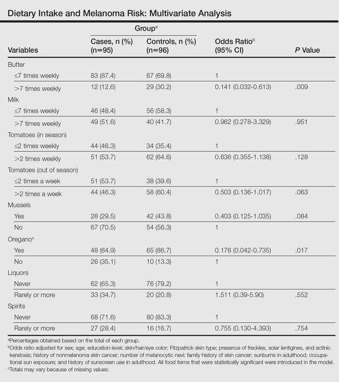
Comment
Observational studies show that diets rich in fruits and vegetables are associated with a lower risk for different types of cancers.7,8 According to some studies, more than 30% of cancers in adulthood could be prevented or delayed by appropriate dietary intake and physical activity.10 However, there are still limited data on some specific cancers such as CM.
Substantial differences in the incidence of CM among different populations have suggested that environmental factors may play an etiological role in the development of CM and diet could be one of the modifiable risk factors.11-13
Initially, we assessed the already known risk factors for CM, and results showed a significantly increased risk for participants with light brown, blonde, or red hair (P<.0001); light-colored and light brown eyes (P<.0001); Fitzpatrick skin types I and II (P<.0001); positive family history of skin cancer (P=.001); the presence of solar lentigines (P<.001), freckles (P<.001), and actinic keratosis (P<.0001); and high number of nevi (P<.0001). Sunburns in adulthood (P<.001) were associated with an increased risk for CM, and our findings are in agreement with the literature.12
Besides confirming the well-known risk factors for CM, our study also showed that some foods (eg, butter, oregano) may act as important protective factors in CM. It could be argued that the increased risks associated with the well-known risk factors (eg, Fitzpatrick skin type, number of sunburns) might not be as strong and/or could be modulated by dietary factors. To further elucidate this critical issue, we analyzed our data by examining the joint relationship between dietary consumption, individual characteristics, sun exposure, and melanoma. We conducted a multivariable analysis controlling for the well-known risk factors and our findings suggest that both butter and oregano, foods that are rich in vitamins A and D, are independent and protective risk factors for melanoma.
Vitamin A (retinol) is a fat-soluble, organic compound that cannot be synthesized by humans but is necessary for normal physiological function and therefore is classified as an essential nutrient. The main source of vitamin A in the human diet is from retinyl esters, mostly from animal products such as dairy products (eg, butter) as well as from plant-based, provitamin A carotenoids (α-carotene, β-carotene) that can be converted to retinol in the intestines.14
Some case-control studies have investigated the association of vitamin A intake and CM risk, reporting mixed findings. Naldi et al15 found a notable inverse association between vitamin A intake and CM risk. Le Marchand et al16 found no inverse association for carotenoids or retinol. Kirkpatrick et al17 found no evidence of a protective effect for vitamin A or carotenoids on CM. However, the Nurses’ Health Study and the Nurses’ Health Study II reported inverse associations between CM and retinol from foods and dietary supplements.8
Dairy products such as butter contain several components considered to be potentially anticarcinogenic, such as calcium, vitamin D, butyric acid, conjugated linoleic acid, sphingolipids, and probiotic bacteria. Some studies found an inverted association between melanoma and high intake of dairy products or other dietary sources of vitamin D, while some investigators showed no association.6,18
Fortes et al18 assessed the role of diet on CM and found no protective effects of butter intake against the development of melanoma; however, a protective effect was found for carrots, which are rich in provitamin A (β-carotene) and for the regular intake of herbs rich in polyphenols (eg, rosemary). In our study, we found a protective effect against CM for butter but not for other dairy products. These findings could be explained by the high content of vitamin A in butter in comparison to other dairy products. Habitual intake of oregano also was associated with a protective effect for CM. Oregano is rich in polyphenols such as carvacrol, thymol, and rosmarinic acid, which are known for their antioxidant capacities and the inhibition of cyclooxygenase.19-21 At experimental levels, both carvacrol and thymol have been shown to inhibit the growth of melanoma cells.19,20 Rosmarinic acid, contained by both rosemary and oregano, have been shown at experimental levels to have photoprotective effects against melanoma.21
The relationship between dietary and nutritional intake and CM has a great potential that should be further explored. Tong and Young22 showed that proanthocyanidins found in grape seeds, epigallocatechin-3-gallate, resveratrol, rosmarinic acid, lycopene, and fig latex have demonstrated clear anticancer effects toward melanoma.
The strength of this study is the high response rate of both cases and controls and the use of incidence melanoma cases that decrease recall bias. A limitation of our study is that food portions were based on average portion size for each food item and therefore it can capture habitual consumption but not calculate actual nutrient intake. Misclassification of dietary exposure also could be a problem. Part of this misclassification is a result of a food frequency questionnaire being an imperfect measure of dietary history; however, we evaluated the reproducibility of the food frequency questionnaire used in this case-control study. Overall, there was a fair to good reproducibility between answers in 2 different periods (12 months apart). For example, agreement for frequency of intake of fresh herbs, tomatoes, and butter were 90.8%, 83.1%, and 83.3%, respectively.
Our sample size had sufficient statistical power to detect the effects of diet on CM.
Conclusion
Our study indicates that butter and oregano intake seem to have a protective role against the development of CM. Further studies are needed to confirm these findings.
- Gilchrest B, Eller MS, Geller AC, et al. The pathogenesis of melanoma induced by ultraviolet radiation. N Engl J Med. 1999;340:1341-1347.
- Lotti T, Bruscino N, Hercogova J, et al. Controversial issues on melanoma. Dermatol Ther. 2012;25:458-462.
- Ródenas JM, Delgado-Rodríguez M, Herranz MT, et al. Sun exposure, pigmentary traits, and risk of cutaneous malignant melanoma: a case-control study in a Mediterranean population. Cancer Causes Control. 1996;7:275-283.
- Autier P, Doré JF. Influence of sun exposures during childhood and during adulthood on melanoma risk. EEPIMEL and EORTC. Melanoma Cooperative Group. European Organization for research and treatment of cancer. Int J Cancer. 1998;77:533-537.
- Fortes C, Mastroeni S, Melchi F, et al. The association between residential pesticide use and cutaneous melanoma. Eur J Cancer. 2007;43:1066-1075.
- Jensen JD, Wing GJ, Dellavalle RP. Nutrition and melanoma prevention. Clin Dermatol. 2010;28:644-649.
- Millen AE, Tucker MA, Hartge P, et al. Diet and melanoma in a case-control study. Cancer Epidemiol Biomarkers Prev. 2004;13:1042-1051.
- Feskanich D, Willett WC, Hunter DJ, et al. Dietary intakes of vitamins A, C, and E and risk of melanoma in two cohorts of women. Br J Cancer. 2003;88:1381-1387.
- English DR, Mac Lennan R, Rivers J, et al. Epidemiological studies of melanocytic naevi: protocol for identifying and recording naevi. International Agency for Research on Cancer (IARC) internal report. No. 90/002. Lyon, France: IARC; 1990.
- Cancer preventability statistics. World Cancer Research Fund website. http://www.wcrf-uk.org/uk/preventing-cancer/cancer-preventability-statistics. Accessed May 24, 2016.
- Gandini S, Raimondi S, Gnagnarella P, et al. Vitamin D and skin cancer: a meta-analysis. Eur J Cancer. 2009;45:634-641.
- Gandini S, Sera F, Cattaruzza MS, et al. Meta-analysis of risk factors for cutaneous melanoma: II. sun exposure. Eur J Cancer. 2005;41:45-60.
- Volkovova K, Bilanicova D, Bartonova A, et al. Associations between environmental factors and incidence of cutaneous melanoma. review. Environ Health. 2012;11(11, suppl 1):S12.
- Asgari MM, Brasky TM, White E. Association of vitamin A and carotenoid intake with melanoma risk in a large prospective cohort. J Invest Dermatol. 2012;132:1573-1582.
- Naldi L, Gallus S, Tavani A, et al. Risk of melanoma and vitamin A, coffee and alcohol: a case-control study from Italy. Eur J Cancer Prev. 2004;13:503-508.
- Le Marchand L, Saltzman BS, Hankin JH, et al. Sun exposure, diet, and melanoma in Hawaii Caucasians. Am J Epidemiol. 2006;164:232-245.
- Kirkpatrick CS, White E, Lee JA. Case-control study of malignant melanoma in Washington State. II. diet, alcohol, and obesity. Am J Epidemiol. 1994;139:869-880.
- Fortes C, Mastroeni S, Melchi F, et al. A protective effect of the Mediterranean diet for cutaneous melanoma. Int J Epidemiol. 2008;37:1018-1029.
- Landa P, Kokoska L, Pribylova M, et al. In vitro anti-inflammatory activity of carvacrol: inhibitory effect on COX-2 catalyzed prostaglandin E(2) biosynthesis. Arch Pharm Res. 2009;32:75-78.
- He L, Mo H, Hadisusilo S, et al. Isoprenoids suppress the growth of murine B16 melanomas in vitro and in vivo. J Nutr. 1997;127:668-674.
- Sánchez-Campillo M, Gabaldon JA, Castillo J, et al. Rosmarinic acid, a photo-protective agent against UV and other ionizing radiations. Food Chem Toxicol. 2009;47:386-392.
- Tong LX, Young LC. Nutrition: the future of melanoma prevention? J Am Acad Dermatol. 2014;71:151-160.
The incidence of cutaneous melanoma (CM) has increased, warranting further study of new risk factors.1,2 Hereditary risk factors for CM include light-colored eyes; fair skin; light brown, blonde, or red hair; tendency to burn; high density of freckles; history of other types of skin cancer; high number of common, atypical, and/or congenital nevi; and family history of skin cancer, as well as risks related to the presence of CDKN2A, BRAF, and MC1R gene mutations. Environmental risk factors include UV exposure from sunlight or tanning beds, among others.3-5
Nutritional factors also have been suggested as possible modifiable risk factors for CM.6 Evidence from epidemiological studies show that diets rich in fruits and vegetables are associated with lower risks for several types of cancer.7,8 A growing number of studies have assessed the effects of diet and the intake of nutrients on the prevention of cancer, specifically the use of dietary supplements to protect the skin from the adverse effects of UV light.6
Preformed vitamin A (ie, retinol) is necessary for the regulation of cell differentiation and also can reduce the incidence of skin tumors in animals exposed to UV light. Certain carotenoids such as α-carotene and β-carotene are metabolized to retinol. These retinol precursors, along with antioxidant nutrients, are important components of fruits and vegetables and may account for the observed anticancer effects of these foods.8
The aim of this study was to assess the relationship between dietary intake and the risk for CM.
Methods
Participants
A case-control study was carried out between 2012 and 2013 at 3 reference centers in Porto Alegre, Brazil—Universidade Federal de Ciências da Saúde de Porto Alegre, Pontifícia Universidade Católica do Rio Grande do Sul, and Hospital de Clínicas de Porto Alegre—for the treatment of patients with CM. Enrolled patients were 18 years and older with a diagnosis of primary CM confirmed by histology. Controls were selected from patients at the same centers, and they were enrolled and matched by institution. Controls were frequency matched to cases by sex and age (+/– 5 years). Exclusion criteria for controls were those presenting with suspicious lesions and those needing radiation therapy or chemotherapy due to other diseases. The study was approved by the ethics committees of the participating centers and informed consent was obtained from all participants. A total of 191 participants (95 cases; 96 controls) were enrolled in the study.
Data Collection
After informed consent was obtained, participants were interviewed and were clinically examined by an experienced dermatologist (C.B.H. and M.M.S.). The questionnaire included sociodemographic variables, medical history, phenotypic characteristics (ie, Fitzpatrick skin type, skin/hair/eye color), family history of skin cancer, history of sunlight exposure, history of sunburns, use of artificial tanning, sunscreen use, and detailed dietary intake. Physical examination included the assessment of several melanocytic lesions (nevi, freckles/ephelides, lentigines, and café au lait spots), actinic keratoses, solar elastosis, and nonmelanocytic tumors following the International Agency for Research on Cancer (IARC) protocol.9
Using a food frequency questionnaire, participants were asked to report their usual frequency of consumption of each food from a list of 36 foods. The frequency of intake of all groups of food and beverages was defined according to the following scale: never, rarely (less than once monthly), once or twice weekly, 3 to 4 times weekly, 5 to 7 times weekly, and more than 7 times weekly. Combination of categories was based on the overall distribution among controls. Therefore, for some items such as mussels and fresh herbs, only 2 categories were used.
Statistical Analysis
A descriptive statistical analysis of the results was performed using SPSS version 20.0 with absolute and relative frequencies for the categorical variables, and mean, SD, and median for the continuous variables. The symmetry of distributions was investigated using the Kolmogorov-Smirnov test.
A t test for independent groups was applied for the continuous variables, while the Pearson χ2 test was used for the categorical variables. The Fisher exact test was used in situations in which at least 25% of the values of the cells presented an expected frequency of less than 5. Monte Carlo simulation was used when at least 1 variable had a polytomic characteristic. Odds ratio (OR) was used to estimate the strength of the association between exposures and outcome. An unconditional binary logistic regression was used to study the association between dietary variables and the risk for CM. To obtain unbiased estimates, multivariate analyses were performed controlling for 1 or more confounding variables. Using low exposure as a base category, the risks and 95% CIs were calculated for the high-exposure categories. Based on the results of bivariate analyses, variables with P≤.25 or lower were included in the models. The likelihood ratio test was used to decide which covariates should be maintained in the model. To test the goodness of fit of the models, the Hosmer-Lemeshow statistic was used.
Potential confounding factors considered in the logistic regression model were sex; age; education level; skin, hair, and eye color; Fitzpatrick skin type; presence of freckles, solar lentigines, and actinic keratosis; history of nonmelanoma skin cancer; number of melanocytic nevi; family history of skin cancer; sunburns in adulthood (≥6 episodes a year); occupational sun exposure; and history of sunscreen use in adulthood.
Results
A total of 191 participants were enrolled in the study (95 [49.7%] cases; 96 [50.3%] controls). Most participants were female (60.0% of cases; 59.4% of controls). The mean age (SD) of cases and controls was 56.8 (13.9) years and 56.5 (13.2) years, respectively. Mean body mass index (SD) did not differ between cases (27.2 [4.6]) and controls (28.2 [6.5]). Education levels of 8 years or less predominated in both groups (64.2% of cases; 57.3% of controls). No statistical difference was found for sex, age, education, or body mass index. The most frequent anatomic sites of CM were the trunk (54.7%) and arms (20.0%), and the most frequent histological type was superficial spreading (62.8%). The median Breslow thickness was 0.90 mm. Ulceration was observed in 20.9% of the cases, and 67% of participants with CM had a high mitotic rate (≥1 mitosis per square millimeter).
Phenotypic characteristics associated with an increased risk for melanoma were light brown hair (OR, 6.73; 95% CI, 3.30-14.2), blonde/red hair (OR, 21.7; 95% CI, 7.51-63.1), light-colored eyes (eg, blue, gray, green)(OR, 13.2; 95% CI, 6.13-28.7), light brown eyes (OR, 5.01; 95% CI, 2.24-11.5), and Fitzpatrick skin types I and II (OR, 7.37; 95% CI, 2.90-26.1). Family history of skin cancer was associated with an increased risk for CM (OR, 4.31; 95% CI, 1.86-10.7) as well as sunburns in adulthood (OR, 1.64; 95% CI, 1.17-1.99). Regular sunscreen use in adulthood had a 5-fold increased risk for CM compared to not using sunscreen regularly (OR, 5.6; 95% CI, 2.85-10.7). Regarding pigmented lesions, the presence of solar lentigines (OR, 4.8; 95% CI, 2.2-11.2), 60 or more nevi (OR, 5.4; 95% CI, 2.4-12.7), and freckles (OR, 3.7; 95% CI, 1.82-7.64) were all associated with an increased risk for CM. Solar elastosis (OR, 2.5; 95% CI, 1.08-5.85), actinic keratosis (OR, 9.1, 95% CI, 3.97-20.84), and occupational exposure to sun (OR, 2.57; 95% CI, 1.23-5.38) also were associated with an increased risk for melanoma.
The intake of most of the foods and beverages included in the study showed no association with CM. High frequency of butter intake (more than daily) was a protective factor for CM (OR, 0.33; 95% CI, 0.16-0.70) compared to low-frequency consumption (daily and less than daily). Consumption of mussels (OR, 0.53; 95% CI, 0.29-0.97) and oregano (OR, 0.28; 95% CI, 0.12-0.66) also were shown to be protective against CM (OR, 0.53; 95% CI, 0.29-0.97). Regarding beverages, those in the highest categories of consumption—liquor (OR, 2.12; 95% CI, 1.09-4.12) and spirits (OR, 2.23; 95% CI, 1.16-4.68)—were associated with an increased risk for CM.
To identify the relationship between CM and the consumption of some foods that were relevant on bivariate analysis, we performed a multivariate model. When adjustments were made, the association remained for butter (OR, 0.141; 95% CI, 0.032-0.613) and oregano (OR, 0.176; 95% CI, 0.042-0.735), while the risk associated with the consumption of both liquor (OR, 1.511; 95% CI, 0.39-5.90) and spirits (OR, 0.755; 95% CI, 0.130-4.393) disappeared (Table).
Comment
Observational studies show that diets rich in fruits and vegetables are associated with a lower risk for different types of cancers.7,8 According to some studies, more than 30% of cancers in adulthood could be prevented or delayed by appropriate dietary intake and physical activity.10 However, there are still limited data on some specific cancers such as CM.
Substantial differences in the incidence of CM among different populations have suggested that environmental factors may play an etiological role in the development of CM and diet could be one of the modifiable risk factors.11-13
Initially, we assessed the already known risk factors for CM, and results showed a significantly increased risk for participants with light brown, blonde, or red hair (P<.0001); light-colored and light brown eyes (P<.0001); Fitzpatrick skin types I and II (P<.0001); positive family history of skin cancer (P=.001); the presence of solar lentigines (P<.001), freckles (P<.001), and actinic keratosis (P<.0001); and high number of nevi (P<.0001). Sunburns in adulthood (P<.001) were associated with an increased risk for CM, and our findings are in agreement with the literature.12
Besides confirming the well-known risk factors for CM, our study also showed that some foods (eg, butter, oregano) may act as important protective factors in CM. It could be argued that the increased risks associated with the well-known risk factors (eg, Fitzpatrick skin type, number of sunburns) might not be as strong and/or could be modulated by dietary factors. To further elucidate this critical issue, we analyzed our data by examining the joint relationship between dietary consumption, individual characteristics, sun exposure, and melanoma. We conducted a multivariable analysis controlling for the well-known risk factors and our findings suggest that both butter and oregano, foods that are rich in vitamins A and D, are independent and protective risk factors for melanoma.
Vitamin A (retinol) is a fat-soluble, organic compound that cannot be synthesized by humans but is necessary for normal physiological function and therefore is classified as an essential nutrient. The main source of vitamin A in the human diet is from retinyl esters, mostly from animal products such as dairy products (eg, butter) as well as from plant-based, provitamin A carotenoids (α-carotene, β-carotene) that can be converted to retinol in the intestines.14
Some case-control studies have investigated the association of vitamin A intake and CM risk, reporting mixed findings. Naldi et al15 found a notable inverse association between vitamin A intake and CM risk. Le Marchand et al16 found no inverse association for carotenoids or retinol. Kirkpatrick et al17 found no evidence of a protective effect for vitamin A or carotenoids on CM. However, the Nurses’ Health Study and the Nurses’ Health Study II reported inverse associations between CM and retinol from foods and dietary supplements.8
Dairy products such as butter contain several components considered to be potentially anticarcinogenic, such as calcium, vitamin D, butyric acid, conjugated linoleic acid, sphingolipids, and probiotic bacteria. Some studies found an inverted association between melanoma and high intake of dairy products or other dietary sources of vitamin D, while some investigators showed no association.6,18
Fortes et al18 assessed the role of diet on CM and found no protective effects of butter intake against the development of melanoma; however, a protective effect was found for carrots, which are rich in provitamin A (β-carotene) and for the regular intake of herbs rich in polyphenols (eg, rosemary). In our study, we found a protective effect against CM for butter but not for other dairy products. These findings could be explained by the high content of vitamin A in butter in comparison to other dairy products. Habitual intake of oregano also was associated with a protective effect for CM. Oregano is rich in polyphenols such as carvacrol, thymol, and rosmarinic acid, which are known for their antioxidant capacities and the inhibition of cyclooxygenase.19-21 At experimental levels, both carvacrol and thymol have been shown to inhibit the growth of melanoma cells.19,20 Rosmarinic acid, contained by both rosemary and oregano, have been shown at experimental levels to have photoprotective effects against melanoma.21
The relationship between dietary and nutritional intake and CM has a great potential that should be further explored. Tong and Young22 showed that proanthocyanidins found in grape seeds, epigallocatechin-3-gallate, resveratrol, rosmarinic acid, lycopene, and fig latex have demonstrated clear anticancer effects toward melanoma.
The strength of this study is the high response rate of both cases and controls and the use of incidence melanoma cases that decrease recall bias. A limitation of our study is that food portions were based on average portion size for each food item and therefore it can capture habitual consumption but not calculate actual nutrient intake. Misclassification of dietary exposure also could be a problem. Part of this misclassification is a result of a food frequency questionnaire being an imperfect measure of dietary history; however, we evaluated the reproducibility of the food frequency questionnaire used in this case-control study. Overall, there was a fair to good reproducibility between answers in 2 different periods (12 months apart). For example, agreement for frequency of intake of fresh herbs, tomatoes, and butter were 90.8%, 83.1%, and 83.3%, respectively.
Our sample size had sufficient statistical power to detect the effects of diet on CM.
Conclusion
Our study indicates that butter and oregano intake seem to have a protective role against the development of CM. Further studies are needed to confirm these findings.
- Gilchrest B, Eller MS, Geller AC, et al. The pathogenesis of melanoma induced by ultraviolet radiation. N Engl J Med. 1999;340:1341-1347.
- Lotti T, Bruscino N, Hercogova J, et al. Controversial issues on melanoma. Dermatol Ther. 2012;25:458-462.
- Ródenas JM, Delgado-Rodríguez M, Herranz MT, et al. Sun exposure, pigmentary traits, and risk of cutaneous malignant melanoma: a case-control study in a Mediterranean population. Cancer Causes Control. 1996;7:275-283.
- Autier P, Doré JF. Influence of sun exposures during childhood and during adulthood on melanoma risk. EEPIMEL and EORTC. Melanoma Cooperative Group. European Organization for research and treatment of cancer. Int J Cancer. 1998;77:533-537.
- Fortes C, Mastroeni S, Melchi F, et al. The association between residential pesticide use and cutaneous melanoma. Eur J Cancer. 2007;43:1066-1075.
- Jensen JD, Wing GJ, Dellavalle RP. Nutrition and melanoma prevention. Clin Dermatol. 2010;28:644-649.
- Millen AE, Tucker MA, Hartge P, et al. Diet and melanoma in a case-control study. Cancer Epidemiol Biomarkers Prev. 2004;13:1042-1051.
- Feskanich D, Willett WC, Hunter DJ, et al. Dietary intakes of vitamins A, C, and E and risk of melanoma in two cohorts of women. Br J Cancer. 2003;88:1381-1387.
- English DR, Mac Lennan R, Rivers J, et al. Epidemiological studies of melanocytic naevi: protocol for identifying and recording naevi. International Agency for Research on Cancer (IARC) internal report. No. 90/002. Lyon, France: IARC; 1990.
- Cancer preventability statistics. World Cancer Research Fund website. http://www.wcrf-uk.org/uk/preventing-cancer/cancer-preventability-statistics. Accessed May 24, 2016.
- Gandini S, Raimondi S, Gnagnarella P, et al. Vitamin D and skin cancer: a meta-analysis. Eur J Cancer. 2009;45:634-641.
- Gandini S, Sera F, Cattaruzza MS, et al. Meta-analysis of risk factors for cutaneous melanoma: II. sun exposure. Eur J Cancer. 2005;41:45-60.
- Volkovova K, Bilanicova D, Bartonova A, et al. Associations between environmental factors and incidence of cutaneous melanoma. review. Environ Health. 2012;11(11, suppl 1):S12.
- Asgari MM, Brasky TM, White E. Association of vitamin A and carotenoid intake with melanoma risk in a large prospective cohort. J Invest Dermatol. 2012;132:1573-1582.
- Naldi L, Gallus S, Tavani A, et al. Risk of melanoma and vitamin A, coffee and alcohol: a case-control study from Italy. Eur J Cancer Prev. 2004;13:503-508.
- Le Marchand L, Saltzman BS, Hankin JH, et al. Sun exposure, diet, and melanoma in Hawaii Caucasians. Am J Epidemiol. 2006;164:232-245.
- Kirkpatrick CS, White E, Lee JA. Case-control study of malignant melanoma in Washington State. II. diet, alcohol, and obesity. Am J Epidemiol. 1994;139:869-880.
- Fortes C, Mastroeni S, Melchi F, et al. A protective effect of the Mediterranean diet for cutaneous melanoma. Int J Epidemiol. 2008;37:1018-1029.
- Landa P, Kokoska L, Pribylova M, et al. In vitro anti-inflammatory activity of carvacrol: inhibitory effect on COX-2 catalyzed prostaglandin E(2) biosynthesis. Arch Pharm Res. 2009;32:75-78.
- He L, Mo H, Hadisusilo S, et al. Isoprenoids suppress the growth of murine B16 melanomas in vitro and in vivo. J Nutr. 1997;127:668-674.
- Sánchez-Campillo M, Gabaldon JA, Castillo J, et al. Rosmarinic acid, a photo-protective agent against UV and other ionizing radiations. Food Chem Toxicol. 2009;47:386-392.
- Tong LX, Young LC. Nutrition: the future of melanoma prevention? J Am Acad Dermatol. 2014;71:151-160.
Practice Points
- Hereditary and environmental risk factors have been identified for cutaneous melanoma (CM). Nutritional factors have been suggested as possible modifiable risk factors.
- Foods rich in vitamins A and D may be protective risk factors for CM.

E-cigarettes: Who’s using them and why?
ABSTRACT
Background Electronic cigarettes (e-cigarettes) are often marketed as safe and effective aids for quitting cigarette smoking, but concerns remain that use of e-cigarettes might actually reduce the number of quit attempts. To address these issues, we characterized the utilization and demographic correlates of dual use of e-cigarettes and traditional cigarettes (referred to here as simply “cigarettes”) among smokers in a rural population of Illinois.
Methods The majority of survey participants were recruited from the 2014 Illinois State Fair and from another event—the Springfield Mile (a motorcycle racing event)—in Springfield, Ill. Survey questions explored participant demographics and cigarette and e-cigarette use history.
Results Of 201 total cigarette smokers, 79 smoked only tobacco cigarettes (smokers), while 122 also used e-cigarettes (dual users). Dual users did not differ significantly from smokers in gender, age, income, or education. Compared to smokers, dual users were more likely to smoke within 30 minutes of awakening (odds ratio [OR]=3.3; 95% confidence interval [CI], 1.8-6.3), but did not smoke more cigarettes per day or perceive a greater likelihood of quit success. Non-white dual users smoked fewer cigarettes per day than smokers. In addition, 79.5% of all dual users reported that they were using e-cigarettes to quit smoking or reduce the number of cigarettes smoked, and white respondents were 6 times more likely than non-whites to use e-cigarettes for ‘trying to quit smoking’ (OR=6.0; 95% CI, 1.1-32.9). Males and respondents with lower income were less likely to say they were using e-cigarettes to reduce the number of cigarettes smoked than females or participants with higher income (OR=0.2; 95% CI, 0.1-0.8 and OR=0.1; 95% CI, 0.0-0.5, respectively).
Conclusions E-cigarettes may significantly alter the landscape of nicotine physical dependence, and local influences likely are associated with use patterns. Future research should continue to examine whether dual use of traditional and electronic cigarettes impacts smoking cessation, and clinicians should be aware that local norms may create differences from national level data.
Approximately 21% of US adults use tobacco products at least occasionally.1 Although smoking prevalence has declined in recent years (from 21% in 2005 to 18% in 2013), it remains high among certain groups (eg, males and those with a high school education or less).2 As we know, the health burden of smoking—as a cause of death from cancer, pulmonary disease, and heart disease—is substantial,3,4 and rural areas experience a significantly higher prevalence of smoking compared to urban areas.2,5,6
However, it is unknown if the context and habits surrounding tobacco use in rural and/or Midwestern areas are similar to those of urban or nationally-representative populations. For example, while many urban residents may encounter a multitude of media messages encouraging smoking cessation resulting in less community acceptance of smoking, rural residents may be exposed to substantially fewer messages (eg, no city bus signs, billboards, subway posters, etc.) and the community may be more accommodating and tolerant of smoking.
Do e-cigarettes increase cigarette smoking?
Public health professionals are concerned about the increased use of e-cigarettes, particularly among young people, and whether this use increases the likelihood that individuals will start smoking tobacco cigarettes.7(Throughout this paper, we will use “cigarettes” and “smoking” to refer to the use of traditional tobacco cigarettes.) A recent study found that adolescents who used electronic nicotine delivery systems were twice as likely as non-users to have tried cigarettes in the past year.8
An onslaught of advertising. There are also concerns that e-cigarettes may serve to ‘renormalize’ nicotine addiction, in part through large-scale advertising, which was seen by nearly 70% of the participants in the 2014 National Youth Tobacco Survey.9 Largely as a result of that advertising, e-cigarette sales exceed $1.7 billion in the United States alone.10 With 15% of all US adults having ever tried electronic nicotine delivery systems and more than half (52%) of smokers having done so, questions regarding their health impact cannot be taken lightly.11
Do e-cigarettes help people quit smoking? E-cigarettes are often marketed as a safe and effective means for quitting cigarette smoking.12-14 (See "E-cigarettes: How "safe" are they?") Nearly two-thirds of physicians report being asked about e-cigarettes by their patients and approximately one-third of physicians recommend using them as a smoking cessation aid.15
Claims regarding the usefulness of e-cigarettes in smoking cessation, however, have not been substantiated by high-quality randomized controlled trials (RCTs). In fact, no RCTs have shown them to be safer or more effective than cessation treatments currently approved by the US Food and Drug Administration.16,17
Two studies reflect the conflicting data that are currently available. One small study found intensive e-cigarette users were 6 times more likely than non-users/triers to report successful smoking cessation.18 However, researchers surveying callers of a cigarette quit line found that smokers who used e-cigarettes (dual users) were less likely to quit smoking than non-users.19
The lack of good-quality data substantiates the concern that dual use might discourage quitting by normalizing cigarette use and reducing perceptions of harm.20,21 Dual use may also hamper smoking cessation efforts by increasing nicotine physical dependence and associated withdrawal symptoms when trying to quit.22 And finally, dual use may expose users to more carcinogens and toxins than those who use only one product, and the average number of cigarettes smoked per day may be significantly higher among dual users.23
Unique demographic factors at work? Finally, the social and community context within which smoking occurs, and the prevalence of smoking-associated demographic risk factors, may vary significantly between rural and urban areas and between seemingly similar rural areas.24-27 Few studies have examined differences in e-cigarette use between rural and urban areas. Those that have are contradictory, reporting that rural residents use e-cigarettes both more and less than their urban peers,28,29 but many of these studies were conducted outside the United States, where the context and norms associated with smoking and e-cigarette use likely vary.
For these reasons, we sought to examine e-cigarette use among residents of Illinois, the nation’s fifth largest state and one with a rural population exceeding 1.5 million.30 We compared dual users of e-cigarettes and cigarettes to smokers of cigarettes only in terms of demographic characteristics, nicotine physical dependence, and smoking cessation beliefs, and explored dual smokers' reasons for using both types of cigarettes.
MATERIALS AND METHODS
A survey was fielded during August and September 2014 in Springfield, Ill. To obtain responses, a booth was set up at both the Illinois State Fair and the Springfield Mile (a motorcycle racing event), and participants were recruited via direct solicitation by project staff. This was supplemented by an email invitation to all employees of the Southern Illinois University School of Medicine. The 2 venues and the email strategy were chosen because they draw from a large area of central and southern Illinois and were convenient to the location of the study team. Individuals were eligible to participate if they were ≥18 years of age and used any tobacco product or e-cigarettes. Survey elements were derived from 2 national surveys of health and behavior—the Minnesota Adult Tobacco Survey 201031 and the Brief Smoking Consequences Questionnaire-Adult.32
Survey questions assessed cigarette use, nicotine physical dependence, social norms, perceived risks and benefits, and smoking cessation beliefs and behaviors. Questions were slightly reworded to address not only the use of traditional cigarettes, but the use of e-cigarettes, as well. Ultimately, each participant answered a similarly-worded set of questions for both regular and e-cigarettes. Dual use of cigarettes and e-cigarettes was also assessed. Participants self-reported all data and survey responses on an electronic tablet and received a $10 (cash or gift card) incentive. This project was reviewed and approved by the Springfield Committee for Research Involving Human Subjects.
Stratification of results. Race was dichotomized into white and non-white. Education was stratified into 3 categories: up to and including high school graduation, some college but not a Bachelor’s degree, and Bachelor’s degree and above. Income was divided as being ≤$20,000 or >$20,000, and age was split into 2 groups by the median value. Analyses included descriptions of participant demographics, dual use status, measures of nicotine physical dependence, quit attempts, and e-cigarette use motivations. Bivariate relationships between dual use status and demographic characteristics, nicotine physical dependence, and smoking cessation beliefs were analyzed by chi-square (categorical variables) and ANOVA (continuous/Likert variables).
Multivariable logistic regression modeling of the demographic variables and dual use status (cigarette smoker only vs dual user) was performed to predict 3 factors: number of cigarettes smoked per day (≤10 vs 11+); time to first cigarette (≤30 vs 31+ minutes from waking); and perceived likelihood of quit attempt success (very/somewhat likely vs very/somewhat unlikely). Multivariable models examining the reasons for dual use included the demographic, nicotine physical dependence, and cessation belief items described previously.
RESULTS
Of 309 total survey participants (Fair=288; Race=12; Email=9), there were 235 current cigarette smokers consisting of 79 who smoked only cigarettes (smokers); 122 who used both cigarettes and e-cigarettes (dual users); and 34 former e-cigarette users. Only smokers and dual users were included in this analysis (N=201, although for the purposes of TABLE 1, N=200 or 199 because at least one participant did not provide answers to all of the questions). Approximately 51% of the smokers were male, 78% were white, 12% were 4-year college graduates, and 57% reported incomes >$20,000. The mean age was 37.7 years (SD=14.4); 50% of respondents were <35 years of age. Dual users did not vary significantly from smokers in terms of gender, age, education, or income (all P>.05). However, a greater proportion of whites vs non-whites were dual users (54.9% vs 42.3%; P=.035).
Click here to see an enlarged version of the table.
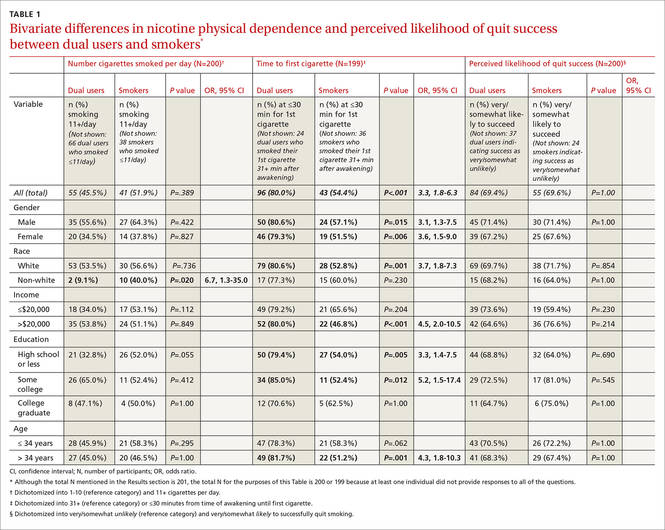
No big quit differences. Bivariate analyses revealed that dual users were no more likely than smokers to have attempted to quit smoking within the past year (X2=2.3; P=.14), consider quitting in the next one or 6 months (X2=1.1; P=.34), or differ in perceived likelihood of cessation success (X2=0.0; P=1.00). The proportion of dual users who smoked 11+ cigarettes per day did not differ from that of cigarette smokers for the group as a whole or when the group was stratified by gender, income, education, or age. However, among non-whites, dual users smoked fewer cigarettes than cigarette smokers (TABLE 1).
Predicting physical dependence. Significant differences also were observed regarding the timing of the first cigarette of the day, with dual users approximately 3 times more likely than smokers to smoke within 30 minutes of awakening (80% vs 54.4%; OR=3.3; 95% CI, 1.8-6.3), and this difference was upheld among males, females, whites, those with an income >$20,000, those with a high school education or less and those with some college education, and age >34 years. There was no association, however, between dual use and perceived likelihood of quit success.
We then performed multivariable logistic modeling on dual users to determine which variables might predict 3 measures of physical dependence: number of cigarettes smoked per day (≤10 vs 11+), time between waking and smoking the first cigarette of the day (≤30 vs 31+ minutes), and perceived likelihood of cessation success (TABLE 2). Male gender (OR=3.4; 95% CI, 1.8-6.5) and white race (OR=4.4; 95% CI, 1.9-10.1) were significant for predicting smoking 11+ cigarettes a day, while dual use status was insignificant (P=.104). Regarding time to first cigarette, only dual use was significant (OR=3.1; 95% CI, 1.6-5.9), with dual users approximately 3 times more likely than smokers to have their first cigarette within 30 minutes of waking. No variables were significant in predicting perceived likelihood of quit success.
Reasons for dual use. We examined reasons for dual use with the question: Do you use e-cigarettes to reduce your regular tobacco use? Here, 79.5% of smokers reported using e-cigarettes to quit smoking or reduce the number of cigarettes smoked.
A multivariable polynomial logistic regression that included only dual users was performed to examine which variables might predict use for tobacco cessation (“trying to quit smoking”) vs reduction in smoking intensity (“trying to reduce the number of regular cigarettes I smoke per day”) vs no change (“use the same amount of tobacco as always”) (TABLE 2). Whites were approximately 6 times more likely than non-whites to indicate they engage in dual use to try to quit smoking (OR=6.0; 95% CI, 1.1-32.9). Males and people with lower incomes were much less likely to indicate they engaged in dual use to try to reduce the number of regular cigarettes smoked than females or those with higher incomes (OR=0.2; 95% CI, 0.1-0.8 and OR=0.1, 95% CI, 0.0-0.5, respectively). No other demographic variables or measures of nicotine physical dependence were significantly different between dual users and smokers.
Click here to see an enlarged version of the table.
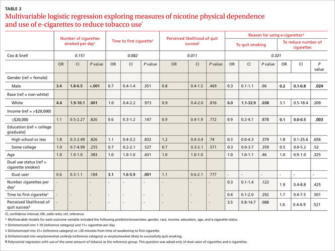
DISCUSSION
E-cigarettes are used by approximately half of smokers (52%), which is much higher than that reported by Delnevo, et al, in their analysis of the National Health Interview Study.33 There, prevalence of dual use of both cigarettes and e-cigarettes ranged from 3.4% to 12.7%. This substantial difference raises important questions regarding study population characterization. Were participants in our study representative of central Illinois, state fair attendees, or the agricultural profession? Further work to identify this group with an increased propensity for dual use will assist clinicians in developing appropriate intervention strategies.
Dual use in our study did not vary by many customary demographic variables. Nor was it associated with different rates of past or future quit attempts or perceived ability to successfully quit if quitting was attempted. These factors—high rates of dual use and insignificant effect on quit attempts—may have implications for local physicians counseling patients who smoke.
In our study, the majority of smokers already use e-cigarettes, and this does not seem to increase their ability/likelihood to quit smoking. Further, dual use did not seem to be associated with overall cigarette consumption; males and white participants smoked more cigarettes than females and non-whites. But dual use was associated with a measure of increased nicotine physical dependence (earlier first cigarette of the day). As a result, physicians may want to think twice before recommending e-cigarette use as a means of smoking cessation.
In addition to the high prevalence of e-cigarette use among smokers, a number of other interesting findings surfaced that run counter to some of the current literature. First, dual users are no more likely than smokers to have tried to quit in the past or to try to quit in the future.21,22,34 It could be that for the relatively small geographical area from which our participants were recruited (central Illinois; ~77% of participants from Sangamon County alone), the local context and culture of smoking differs from that associated with participants in other studies, who were mostly recruited from national and regional online surveys. However, there is no a priori reason to suspect Sangamon County is especially different, as it is quite similar to Illinois as a whole by many measures (eg, percentage rural: 14.1% vs 11.5%; percentage black (only): 12.4% vs 14.7%; education to at least a Bachelor’s degree: 33.0% vs 31.9%; and median household income: $55,565 vs $57,166).30
While we found that dual users did have one measure of increased nicotine physical dependence, the total number of cigarettes consumed per day was not significantly different from that of smokers.23-25 This is contrary to another study of nicotine physical dependence, but, unlike that study, we did not assess length of time of concurrent use.35 There is much uncertainty surrounding the issue of nicotine physical dependence and e-cigarette use, largely because the level of nicotine delivered by various e-products varies significantly.36
Cross-sectional nature, small sample size limit utility of data
There are significant limitations to this study, including the cross-sectional nature of the data, the small sample size, the use of self-report, and the limited scope of recruitment. The relatively small sample size limits our ability to observe small differences and effect sizes. However, small differences often lack practical significance. Finally, participation was limited to those attending a state fair or a local sporting event and those employed by a local medical school. Thus, the results may not be generalizable to populations outside central Illinois. On the other hand, the very low income sample recruited from the Midwestern US, which is underrepresented in prior e-cigarette research, might represent some of the strengths of this work.
Future investigations. Future studies should more closely examine e-cigarette use prevalence on smaller geographic scales and especially in rural areas where there is a paucity of research. As the majority of our respondents came from a single county in central Illinois, one has to ask the questions, “Is this a ‘hot spot’ for e-cigarette use?" And "Do other rural areas experience similar use?” It may be important to know if national surveys are sensitive enough to observe significant local variations. Research also should examine how e-cigarette use and the influence of local culture vary across wider areas.
Several specific areas of study would help to inform policy and intervention development. For example, is tobacco cigarette quit success impacted by concurrent e-cigarette use? While our study showed no difference in past or possible future quit attempts among dual users as compared with smokers, we did not assess actual quit success, and multiple participants in our study anecdotally described using e-cigarettes to successfully quit smoking.
In the end, the rapid increase in the use of e-cigarettes has the potential to significantly alter the landscape of nicotine physical dependence, and local culture and other influences are likely associated with use patterns.
CORRESPONDENCE
Wiley D. Jenkins, PhD, MPH, Science Director, Population Health Science Program, Southern Illinois University School of Medicine, 201 E. Madison St., Springfield, IL 62794-9664; [email protected].
1. Agaku IT, King BA, Husten CG, et al; Centers for Disease Control and Prevention (CDC). Tobacco product use among adults—United States, 2012-2013. MMWR Morb Mortal Wkly Rep. 2014;63:542-547.
2. Jamal A, Agaku IT, O’Connor E, et al. Current cigarette smoking among adults—United States, 2005-2013. MMWR Morb Mortal Wkly Rep. 2014;63:1108-1112.
3. Siegel RL, Jacobs EJ, Newton CC, et al. Deaths due to cigarette smoking for 12 smoking-related cancers in the United States. JAMA Intern Med. 2015;175:1574-1576.
4. US Department of Health and Human Services. Surgeon General. The Health Consequences of Smoking—50 Years of Progress: A Report of the Surgeon General, 2014. Available at: http://www.surgeongeneral.gov/library/reports/50-years-of-progress/index.html. Accessed January 22, 2014.
5. Gamm LD, Hutchison LL, Dabney BJ, et al, eds. (2003). Rural Healthy People 2010: A companion document to Healthy People 2010. Volume 2. College Station, TX: The Texas A&M University System Health Science Center, School of Rural Public Health, Southwest Rural Health Research Center.
6. Doescher MP, Jackson JE, Jerant A, et al. Prevalence and trends in smoking: a national rural study. J Rural Health. 2006;22:112-118.
7. Bunnell RE, Agaku IT, Arrazola RA, et al. Intentions to smoke cigarettes among never-smoking US middle and high school electronic cigarette users: National Youth Tobacco Survey, 2011-2013. Nicotine Tob Res. 2015;17:228-235.
8. Cardenas VM, Evans VL, Balamurugan A, et al. Use of electronic nicotine delivery systems and recent initiation of smoking among US youth. Int J Public Health. 2016;61:237-241.
9. Auf R, Trepka MJ, Cano MA, et al. Electronic cigarettes: the renormalisation of nicotine use. BMJ. 2016;352:i425.
10. CNBC. E-cigarette sales are smoking hot, set to hit $1.7 billion. Available at: http://www.cnbc.com/id/100991511. Accessed April 5, 2016.
11. Weaver SR, Majeed BA, Pechacek TF, et al. Use of electronic nicotine delivery systems and other tobacco products among USA adults, 2014: results from a national survey. Int J Public Health. 2016;61:177-188.
12. Richardson A, Ganz O, Vallone D. Tobacco on the web: surveillance and characterisation of online tobacco and e-cigarette advertising. Tob Control. 2015;24:341-347.
13. Paek HJ, Kim S, Hove T, et al. Reduced harm or another gateway to smoking? source, message, and information characteristics of E-cigarette videos on YouTube. J Health Commun. 2014;19:545-560.
14. Kim AE, Arnold KY, Makarenko O. E-cigarette advertising expenditures in the U.S., 2011-2012. Am J Prev Med. 2014;46:409-412.
15. Steinberg MB, Giovenco DP, Delnevo CD. Patient-physician communication regarding electronic cigarettes. Prev Med Rep. 2015;2:96-98.
16. Gualano MR, Passi S, Bert F, et al. Electronic cigarettes: assessing the efficacy and the adverse effects through a systematic review of published studies. J Public Health (Oxf). 2015:37:488-497.
17. U.S. National Institutes of Health. ClinicalTrials.gov. Available at: https://clinicaltrials.gov/ct2/results?term=%22electronic+cigarette%22&Search=Search. Accessed July 10, 2015.
18. Biener L, Hargraves JL. A longitudinal study of electronic cigarette use among a population-based sample of adult smokers: association with smoking cessation and motivation to quit. Nicotine Tob Res. 2015;17:127-133.
19. Vickerman KA, Carpenter KM, Altman T, et al. Use of electronic cigarettes among state tobacco cessation quitline callers. Nicotine Tob Res. 2013;15:1787-1791.
20. Center for Disease Control and Prevention. Press Release February 28,2013. Available at: http://www.cdc.gov/media/releases/2013/p0228_electronic_cigarettes.html. Accessed July 8, 2015.
21. Pisinger C. Why public health people are more worried than excited over e-cigarettes. BMC Med. 2014;12:226.
22. Post A, Gilljam H, Rosendahl I, et al. Symptoms of nicotine dependence in a cohort of Swedish youths: a comparison between smokers, smokeless tobacco users and dual tobacco users. Addiction. 2010;105:740-746.
23. Mazurek JM, Syamlal G, King BA, et al; Division of Respiratory Disease Studies, National Institute for Occupational Safety and Health, CDC. Smokeless tobacco use among working adults—United States, 2005 and 2010. MMWR Morb Mortal Wkly Rep. 2014;63:477-482.
24. Hutcheson TD, Greiner KA, Ellerbeck EF, et al. Understanding smoking cessation in rural communities. J Rural Health. 2008;24:116-124.
25. McMillen R, Breen J, Cosby AG. Rural-urban differences in the social climate surrounding environmental tobacco smoke: a report from the 2002 Social Climate Survey of Tobacco Control. J Rural Health. 2004;20:7-16.
26. Butler KM, Rayens MK, Adkins S, et al. Culturally-specific smoking cessation outreach in a rural community. Public Health Nurs. 2014;31:44-54.
27. Butler KM, Hedgecock S, Record RA, et al. An evidence-based cessation strategy using rural smokers’ experiences with tobacco. Nurs Clin North Am. 2012;47:31-43.
28. Hamilton HA, Ferrence R, Boak A, et al. Ever use of nicotine and nonnicotine electronic cigarettes among high school students in Ontario, Canada. Nicotine Tob Res. 2015;17:1212-1218.
29. Goniewicz ML, Zielinska-Danch W. Electronic cigarette use among teenagers and young adults in Poland. Pediatrics. 2012;130:e879-e885.
30. US Census Bureau. 2010 Census Urban and Rural Classification and Urban Area Criteria. Available at: http://www.census.gov/geo/reference/ua/urban-rural-2010.html. Accessed March 13, 2016.
31. Minnesota Adult Tobacco Survey. Tobacco use in Minnesota: 1999-2014. Available at: http://www.mnadulttobaccosurvey.org/. Accessed April 27, 2016.
32. Rash CJ, Copeland AL. The Brief Smoking Consequences Questionnaire-Adult (BSCQ-A): development of a short form of the SCQ-A. Nicotine Tob Res. 2008;10:1633-1643.
33. Delnevo CD, Giovenco DP, Steinberg MB, et al. Patterns of electronic cigarette use among adults in the United States. Nicotine Tob Res. 2016;18:715-719.
34. Lee YO, Hebert CJ, Nonnemaker JM, et al. Multiple tobacco product use among adults in the United States: cigarettes, cigars, electronic cigarettes, hookah, smokeless tobacco, and snus. Prev Med. 2014;62:14-19.
35. Etter JF, Eissenberg T. Dependence levels in users of electronic cigarettes, nicotine gums and tobacco cigarettes. Drug Alcohol Depend. 2015;147:68-75.
36. Cobb CO, Hendricks PS, Eissenberg T. Electronic cigarettes and nicotine dependence: evolving products, evolving problems. BMC Med. 2015;13:119.
ABSTRACT
Background Electronic cigarettes (e-cigarettes) are often marketed as safe and effective aids for quitting cigarette smoking, but concerns remain that use of e-cigarettes might actually reduce the number of quit attempts. To address these issues, we characterized the utilization and demographic correlates of dual use of e-cigarettes and traditional cigarettes (referred to here as simply “cigarettes”) among smokers in a rural population of Illinois.
Methods The majority of survey participants were recruited from the 2014 Illinois State Fair and from another event—the Springfield Mile (a motorcycle racing event)—in Springfield, Ill. Survey questions explored participant demographics and cigarette and e-cigarette use history.
Results Of 201 total cigarette smokers, 79 smoked only tobacco cigarettes (smokers), while 122 also used e-cigarettes (dual users). Dual users did not differ significantly from smokers in gender, age, income, or education. Compared to smokers, dual users were more likely to smoke within 30 minutes of awakening (odds ratio [OR]=3.3; 95% confidence interval [CI], 1.8-6.3), but did not smoke more cigarettes per day or perceive a greater likelihood of quit success. Non-white dual users smoked fewer cigarettes per day than smokers. In addition, 79.5% of all dual users reported that they were using e-cigarettes to quit smoking or reduce the number of cigarettes smoked, and white respondents were 6 times more likely than non-whites to use e-cigarettes for ‘trying to quit smoking’ (OR=6.0; 95% CI, 1.1-32.9). Males and respondents with lower income were less likely to say they were using e-cigarettes to reduce the number of cigarettes smoked than females or participants with higher income (OR=0.2; 95% CI, 0.1-0.8 and OR=0.1; 95% CI, 0.0-0.5, respectively).
Conclusions E-cigarettes may significantly alter the landscape of nicotine physical dependence, and local influences likely are associated with use patterns. Future research should continue to examine whether dual use of traditional and electronic cigarettes impacts smoking cessation, and clinicians should be aware that local norms may create differences from national level data.
Approximately 21% of US adults use tobacco products at least occasionally.1 Although smoking prevalence has declined in recent years (from 21% in 2005 to 18% in 2013), it remains high among certain groups (eg, males and those with a high school education or less).2 As we know, the health burden of smoking—as a cause of death from cancer, pulmonary disease, and heart disease—is substantial,3,4 and rural areas experience a significantly higher prevalence of smoking compared to urban areas.2,5,6
However, it is unknown if the context and habits surrounding tobacco use in rural and/or Midwestern areas are similar to those of urban or nationally-representative populations. For example, while many urban residents may encounter a multitude of media messages encouraging smoking cessation resulting in less community acceptance of smoking, rural residents may be exposed to substantially fewer messages (eg, no city bus signs, billboards, subway posters, etc.) and the community may be more accommodating and tolerant of smoking.
Do e-cigarettes increase cigarette smoking?
Public health professionals are concerned about the increased use of e-cigarettes, particularly among young people, and whether this use increases the likelihood that individuals will start smoking tobacco cigarettes.7(Throughout this paper, we will use “cigarettes” and “smoking” to refer to the use of traditional tobacco cigarettes.) A recent study found that adolescents who used electronic nicotine delivery systems were twice as likely as non-users to have tried cigarettes in the past year.8
An onslaught of advertising. There are also concerns that e-cigarettes may serve to ‘renormalize’ nicotine addiction, in part through large-scale advertising, which was seen by nearly 70% of the participants in the 2014 National Youth Tobacco Survey.9 Largely as a result of that advertising, e-cigarette sales exceed $1.7 billion in the United States alone.10 With 15% of all US adults having ever tried electronic nicotine delivery systems and more than half (52%) of smokers having done so, questions regarding their health impact cannot be taken lightly.11
Do e-cigarettes help people quit smoking? E-cigarettes are often marketed as a safe and effective means for quitting cigarette smoking.12-14 (See "E-cigarettes: How "safe" are they?") Nearly two-thirds of physicians report being asked about e-cigarettes by their patients and approximately one-third of physicians recommend using them as a smoking cessation aid.15
Claims regarding the usefulness of e-cigarettes in smoking cessation, however, have not been substantiated by high-quality randomized controlled trials (RCTs). In fact, no RCTs have shown them to be safer or more effective than cessation treatments currently approved by the US Food and Drug Administration.16,17
Two studies reflect the conflicting data that are currently available. One small study found intensive e-cigarette users were 6 times more likely than non-users/triers to report successful smoking cessation.18 However, researchers surveying callers of a cigarette quit line found that smokers who used e-cigarettes (dual users) were less likely to quit smoking than non-users.19
The lack of good-quality data substantiates the concern that dual use might discourage quitting by normalizing cigarette use and reducing perceptions of harm.20,21 Dual use may also hamper smoking cessation efforts by increasing nicotine physical dependence and associated withdrawal symptoms when trying to quit.22 And finally, dual use may expose users to more carcinogens and toxins than those who use only one product, and the average number of cigarettes smoked per day may be significantly higher among dual users.23
Unique demographic factors at work? Finally, the social and community context within which smoking occurs, and the prevalence of smoking-associated demographic risk factors, may vary significantly between rural and urban areas and between seemingly similar rural areas.24-27 Few studies have examined differences in e-cigarette use between rural and urban areas. Those that have are contradictory, reporting that rural residents use e-cigarettes both more and less than their urban peers,28,29 but many of these studies were conducted outside the United States, where the context and norms associated with smoking and e-cigarette use likely vary.
For these reasons, we sought to examine e-cigarette use among residents of Illinois, the nation’s fifth largest state and one with a rural population exceeding 1.5 million.30 We compared dual users of e-cigarettes and cigarettes to smokers of cigarettes only in terms of demographic characteristics, nicotine physical dependence, and smoking cessation beliefs, and explored dual smokers' reasons for using both types of cigarettes.
MATERIALS AND METHODS
A survey was fielded during August and September 2014 in Springfield, Ill. To obtain responses, a booth was set up at both the Illinois State Fair and the Springfield Mile (a motorcycle racing event), and participants were recruited via direct solicitation by project staff. This was supplemented by an email invitation to all employees of the Southern Illinois University School of Medicine. The 2 venues and the email strategy were chosen because they draw from a large area of central and southern Illinois and were convenient to the location of the study team. Individuals were eligible to participate if they were ≥18 years of age and used any tobacco product or e-cigarettes. Survey elements were derived from 2 national surveys of health and behavior—the Minnesota Adult Tobacco Survey 201031 and the Brief Smoking Consequences Questionnaire-Adult.32
Survey questions assessed cigarette use, nicotine physical dependence, social norms, perceived risks and benefits, and smoking cessation beliefs and behaviors. Questions were slightly reworded to address not only the use of traditional cigarettes, but the use of e-cigarettes, as well. Ultimately, each participant answered a similarly-worded set of questions for both regular and e-cigarettes. Dual use of cigarettes and e-cigarettes was also assessed. Participants self-reported all data and survey responses on an electronic tablet and received a $10 (cash or gift card) incentive. This project was reviewed and approved by the Springfield Committee for Research Involving Human Subjects.
Stratification of results. Race was dichotomized into white and non-white. Education was stratified into 3 categories: up to and including high school graduation, some college but not a Bachelor’s degree, and Bachelor’s degree and above. Income was divided as being ≤$20,000 or >$20,000, and age was split into 2 groups by the median value. Analyses included descriptions of participant demographics, dual use status, measures of nicotine physical dependence, quit attempts, and e-cigarette use motivations. Bivariate relationships between dual use status and demographic characteristics, nicotine physical dependence, and smoking cessation beliefs were analyzed by chi-square (categorical variables) and ANOVA (continuous/Likert variables).
Multivariable logistic regression modeling of the demographic variables and dual use status (cigarette smoker only vs dual user) was performed to predict 3 factors: number of cigarettes smoked per day (≤10 vs 11+); time to first cigarette (≤30 vs 31+ minutes from waking); and perceived likelihood of quit attempt success (very/somewhat likely vs very/somewhat unlikely). Multivariable models examining the reasons for dual use included the demographic, nicotine physical dependence, and cessation belief items described previously.
RESULTS
Of 309 total survey participants (Fair=288; Race=12; Email=9), there were 235 current cigarette smokers consisting of 79 who smoked only cigarettes (smokers); 122 who used both cigarettes and e-cigarettes (dual users); and 34 former e-cigarette users. Only smokers and dual users were included in this analysis (N=201, although for the purposes of TABLE 1, N=200 or 199 because at least one participant did not provide answers to all of the questions). Approximately 51% of the smokers were male, 78% were white, 12% were 4-year college graduates, and 57% reported incomes >$20,000. The mean age was 37.7 years (SD=14.4); 50% of respondents were <35 years of age. Dual users did not vary significantly from smokers in terms of gender, age, education, or income (all P>.05). However, a greater proportion of whites vs non-whites were dual users (54.9% vs 42.3%; P=.035).
Click here to see an enlarged version of the table.
No big quit differences. Bivariate analyses revealed that dual users were no more likely than smokers to have attempted to quit smoking within the past year (X2=2.3; P=.14), consider quitting in the next one or 6 months (X2=1.1; P=.34), or differ in perceived likelihood of cessation success (X2=0.0; P=1.00). The proportion of dual users who smoked 11+ cigarettes per day did not differ from that of cigarette smokers for the group as a whole or when the group was stratified by gender, income, education, or age. However, among non-whites, dual users smoked fewer cigarettes than cigarette smokers (TABLE 1).
Predicting physical dependence. Significant differences also were observed regarding the timing of the first cigarette of the day, with dual users approximately 3 times more likely than smokers to smoke within 30 minutes of awakening (80% vs 54.4%; OR=3.3; 95% CI, 1.8-6.3), and this difference was upheld among males, females, whites, those with an income >$20,000, those with a high school education or less and those with some college education, and age >34 years. There was no association, however, between dual use and perceived likelihood of quit success.
We then performed multivariable logistic modeling on dual users to determine which variables might predict 3 measures of physical dependence: number of cigarettes smoked per day (≤10 vs 11+), time between waking and smoking the first cigarette of the day (≤30 vs 31+ minutes), and perceived likelihood of cessation success (TABLE 2). Male gender (OR=3.4; 95% CI, 1.8-6.5) and white race (OR=4.4; 95% CI, 1.9-10.1) were significant for predicting smoking 11+ cigarettes a day, while dual use status was insignificant (P=.104). Regarding time to first cigarette, only dual use was significant (OR=3.1; 95% CI, 1.6-5.9), with dual users approximately 3 times more likely than smokers to have their first cigarette within 30 minutes of waking. No variables were significant in predicting perceived likelihood of quit success.
Reasons for dual use. We examined reasons for dual use with the question: Do you use e-cigarettes to reduce your regular tobacco use? Here, 79.5% of smokers reported using e-cigarettes to quit smoking or reduce the number of cigarettes smoked.
A multivariable polynomial logistic regression that included only dual users was performed to examine which variables might predict use for tobacco cessation (“trying to quit smoking”) vs reduction in smoking intensity (“trying to reduce the number of regular cigarettes I smoke per day”) vs no change (“use the same amount of tobacco as always”) (TABLE 2). Whites were approximately 6 times more likely than non-whites to indicate they engage in dual use to try to quit smoking (OR=6.0; 95% CI, 1.1-32.9). Males and people with lower incomes were much less likely to indicate they engaged in dual use to try to reduce the number of regular cigarettes smoked than females or those with higher incomes (OR=0.2; 95% CI, 0.1-0.8 and OR=0.1, 95% CI, 0.0-0.5, respectively). No other demographic variables or measures of nicotine physical dependence were significantly different between dual users and smokers.
Click here to see an enlarged version of the table.
DISCUSSION
E-cigarettes are used by approximately half of smokers (52%), which is much higher than that reported by Delnevo, et al, in their analysis of the National Health Interview Study.33 There, prevalence of dual use of both cigarettes and e-cigarettes ranged from 3.4% to 12.7%. This substantial difference raises important questions regarding study population characterization. Were participants in our study representative of central Illinois, state fair attendees, or the agricultural profession? Further work to identify this group with an increased propensity for dual use will assist clinicians in developing appropriate intervention strategies.
Dual use in our study did not vary by many customary demographic variables. Nor was it associated with different rates of past or future quit attempts or perceived ability to successfully quit if quitting was attempted. These factors—high rates of dual use and insignificant effect on quit attempts—may have implications for local physicians counseling patients who smoke.
In our study, the majority of smokers already use e-cigarettes, and this does not seem to increase their ability/likelihood to quit smoking. Further, dual use did not seem to be associated with overall cigarette consumption; males and white participants smoked more cigarettes than females and non-whites. But dual use was associated with a measure of increased nicotine physical dependence (earlier first cigarette of the day). As a result, physicians may want to think twice before recommending e-cigarette use as a means of smoking cessation.
In addition to the high prevalence of e-cigarette use among smokers, a number of other interesting findings surfaced that run counter to some of the current literature. First, dual users are no more likely than smokers to have tried to quit in the past or to try to quit in the future.21,22,34 It could be that for the relatively small geographical area from which our participants were recruited (central Illinois; ~77% of participants from Sangamon County alone), the local context and culture of smoking differs from that associated with participants in other studies, who were mostly recruited from national and regional online surveys. However, there is no a priori reason to suspect Sangamon County is especially different, as it is quite similar to Illinois as a whole by many measures (eg, percentage rural: 14.1% vs 11.5%; percentage black (only): 12.4% vs 14.7%; education to at least a Bachelor’s degree: 33.0% vs 31.9%; and median household income: $55,565 vs $57,166).30
While we found that dual users did have one measure of increased nicotine physical dependence, the total number of cigarettes consumed per day was not significantly different from that of smokers.23-25 This is contrary to another study of nicotine physical dependence, but, unlike that study, we did not assess length of time of concurrent use.35 There is much uncertainty surrounding the issue of nicotine physical dependence and e-cigarette use, largely because the level of nicotine delivered by various e-products varies significantly.36
Cross-sectional nature, small sample size limit utility of data
There are significant limitations to this study, including the cross-sectional nature of the data, the small sample size, the use of self-report, and the limited scope of recruitment. The relatively small sample size limits our ability to observe small differences and effect sizes. However, small differences often lack practical significance. Finally, participation was limited to those attending a state fair or a local sporting event and those employed by a local medical school. Thus, the results may not be generalizable to populations outside central Illinois. On the other hand, the very low income sample recruited from the Midwestern US, which is underrepresented in prior e-cigarette research, might represent some of the strengths of this work.
Future investigations. Future studies should more closely examine e-cigarette use prevalence on smaller geographic scales and especially in rural areas where there is a paucity of research. As the majority of our respondents came from a single county in central Illinois, one has to ask the questions, “Is this a ‘hot spot’ for e-cigarette use?" And "Do other rural areas experience similar use?” It may be important to know if national surveys are sensitive enough to observe significant local variations. Research also should examine how e-cigarette use and the influence of local culture vary across wider areas.
Several specific areas of study would help to inform policy and intervention development. For example, is tobacco cigarette quit success impacted by concurrent e-cigarette use? While our study showed no difference in past or possible future quit attempts among dual users as compared with smokers, we did not assess actual quit success, and multiple participants in our study anecdotally described using e-cigarettes to successfully quit smoking.
In the end, the rapid increase in the use of e-cigarettes has the potential to significantly alter the landscape of nicotine physical dependence, and local culture and other influences are likely associated with use patterns.
CORRESPONDENCE
Wiley D. Jenkins, PhD, MPH, Science Director, Population Health Science Program, Southern Illinois University School of Medicine, 201 E. Madison St., Springfield, IL 62794-9664; [email protected].
1. Agaku IT, King BA, Husten CG, et al; Centers for Disease Control and Prevention (CDC). Tobacco product use among adults—United States, 2012-2013. MMWR Morb Mortal Wkly Rep. 2014;63:542-547.
2. Jamal A, Agaku IT, O’Connor E, et al. Current cigarette smoking among adults—United States, 2005-2013. MMWR Morb Mortal Wkly Rep. 2014;63:1108-1112.
3. Siegel RL, Jacobs EJ, Newton CC, et al. Deaths due to cigarette smoking for 12 smoking-related cancers in the United States. JAMA Intern Med. 2015;175:1574-1576.
4. US Department of Health and Human Services. Surgeon General. The Health Consequences of Smoking—50 Years of Progress: A Report of the Surgeon General, 2014. Available at: http://www.surgeongeneral.gov/library/reports/50-years-of-progress/index.html. Accessed January 22, 2014.
5. Gamm LD, Hutchison LL, Dabney BJ, et al, eds. (2003). Rural Healthy People 2010: A companion document to Healthy People 2010. Volume 2. College Station, TX: The Texas A&M University System Health Science Center, School of Rural Public Health, Southwest Rural Health Research Center.
6. Doescher MP, Jackson JE, Jerant A, et al. Prevalence and trends in smoking: a national rural study. J Rural Health. 2006;22:112-118.
7. Bunnell RE, Agaku IT, Arrazola RA, et al. Intentions to smoke cigarettes among never-smoking US middle and high school electronic cigarette users: National Youth Tobacco Survey, 2011-2013. Nicotine Tob Res. 2015;17:228-235.
8. Cardenas VM, Evans VL, Balamurugan A, et al. Use of electronic nicotine delivery systems and recent initiation of smoking among US youth. Int J Public Health. 2016;61:237-241.
9. Auf R, Trepka MJ, Cano MA, et al. Electronic cigarettes: the renormalisation of nicotine use. BMJ. 2016;352:i425.
10. CNBC. E-cigarette sales are smoking hot, set to hit $1.7 billion. Available at: http://www.cnbc.com/id/100991511. Accessed April 5, 2016.
11. Weaver SR, Majeed BA, Pechacek TF, et al. Use of electronic nicotine delivery systems and other tobacco products among USA adults, 2014: results from a national survey. Int J Public Health. 2016;61:177-188.
12. Richardson A, Ganz O, Vallone D. Tobacco on the web: surveillance and characterisation of online tobacco and e-cigarette advertising. Tob Control. 2015;24:341-347.
13. Paek HJ, Kim S, Hove T, et al. Reduced harm or another gateway to smoking? source, message, and information characteristics of E-cigarette videos on YouTube. J Health Commun. 2014;19:545-560.
14. Kim AE, Arnold KY, Makarenko O. E-cigarette advertising expenditures in the U.S., 2011-2012. Am J Prev Med. 2014;46:409-412.
15. Steinberg MB, Giovenco DP, Delnevo CD. Patient-physician communication regarding electronic cigarettes. Prev Med Rep. 2015;2:96-98.
16. Gualano MR, Passi S, Bert F, et al. Electronic cigarettes: assessing the efficacy and the adverse effects through a systematic review of published studies. J Public Health (Oxf). 2015:37:488-497.
17. U.S. National Institutes of Health. ClinicalTrials.gov. Available at: https://clinicaltrials.gov/ct2/results?term=%22electronic+cigarette%22&Search=Search. Accessed July 10, 2015.
18. Biener L, Hargraves JL. A longitudinal study of electronic cigarette use among a population-based sample of adult smokers: association with smoking cessation and motivation to quit. Nicotine Tob Res. 2015;17:127-133.
19. Vickerman KA, Carpenter KM, Altman T, et al. Use of electronic cigarettes among state tobacco cessation quitline callers. Nicotine Tob Res. 2013;15:1787-1791.
20. Center for Disease Control and Prevention. Press Release February 28,2013. Available at: http://www.cdc.gov/media/releases/2013/p0228_electronic_cigarettes.html. Accessed July 8, 2015.
21. Pisinger C. Why public health people are more worried than excited over e-cigarettes. BMC Med. 2014;12:226.
22. Post A, Gilljam H, Rosendahl I, et al. Symptoms of nicotine dependence in a cohort of Swedish youths: a comparison between smokers, smokeless tobacco users and dual tobacco users. Addiction. 2010;105:740-746.
23. Mazurek JM, Syamlal G, King BA, et al; Division of Respiratory Disease Studies, National Institute for Occupational Safety and Health, CDC. Smokeless tobacco use among working adults—United States, 2005 and 2010. MMWR Morb Mortal Wkly Rep. 2014;63:477-482.
24. Hutcheson TD, Greiner KA, Ellerbeck EF, et al. Understanding smoking cessation in rural communities. J Rural Health. 2008;24:116-124.
25. McMillen R, Breen J, Cosby AG. Rural-urban differences in the social climate surrounding environmental tobacco smoke: a report from the 2002 Social Climate Survey of Tobacco Control. J Rural Health. 2004;20:7-16.
26. Butler KM, Rayens MK, Adkins S, et al. Culturally-specific smoking cessation outreach in a rural community. Public Health Nurs. 2014;31:44-54.
27. Butler KM, Hedgecock S, Record RA, et al. An evidence-based cessation strategy using rural smokers’ experiences with tobacco. Nurs Clin North Am. 2012;47:31-43.
28. Hamilton HA, Ferrence R, Boak A, et al. Ever use of nicotine and nonnicotine electronic cigarettes among high school students in Ontario, Canada. Nicotine Tob Res. 2015;17:1212-1218.
29. Goniewicz ML, Zielinska-Danch W. Electronic cigarette use among teenagers and young adults in Poland. Pediatrics. 2012;130:e879-e885.
30. US Census Bureau. 2010 Census Urban and Rural Classification and Urban Area Criteria. Available at: http://www.census.gov/geo/reference/ua/urban-rural-2010.html. Accessed March 13, 2016.
31. Minnesota Adult Tobacco Survey. Tobacco use in Minnesota: 1999-2014. Available at: http://www.mnadulttobaccosurvey.org/. Accessed April 27, 2016.
32. Rash CJ, Copeland AL. The Brief Smoking Consequences Questionnaire-Adult (BSCQ-A): development of a short form of the SCQ-A. Nicotine Tob Res. 2008;10:1633-1643.
33. Delnevo CD, Giovenco DP, Steinberg MB, et al. Patterns of electronic cigarette use among adults in the United States. Nicotine Tob Res. 2016;18:715-719.
34. Lee YO, Hebert CJ, Nonnemaker JM, et al. Multiple tobacco product use among adults in the United States: cigarettes, cigars, electronic cigarettes, hookah, smokeless tobacco, and snus. Prev Med. 2014;62:14-19.
35. Etter JF, Eissenberg T. Dependence levels in users of electronic cigarettes, nicotine gums and tobacco cigarettes. Drug Alcohol Depend. 2015;147:68-75.
36. Cobb CO, Hendricks PS, Eissenberg T. Electronic cigarettes and nicotine dependence: evolving products, evolving problems. BMC Med. 2015;13:119.

Hospice Care Insurance and Readmissions
Palliative care and hospice specialists consult on a variety of patients in the acute care setting that span all diagnoses and specialties. These include patients in the intensive care units, oncology units, as well as patients with end‐stage pulmonary, cardiac, and renal diseases. Discharge of these patients is often complicated by social issues, intensive personal care needs, and decreased functional status, as well as by the patient's insurance. Options for discharge disposition for patients accepting enrollment in hospice are often limited by financial constraints. Medicare pays for a set package of hospice benefits that do not include payment for room and board for hospice residential care and have a limited number of hours for a personal care attendant.[1] Hospice inpatient units are typically covered only for patients with acute care needs. Patients with secondary commercial insurance similarly find that custodial care benefits are often lacking, as most private and managed care plans mimic the Medicare hospice benefit.[2]
Palliative care inpatient consultation and palliative or hospice home care are associated with decreased 30‐day readmission rates.[3, 4, 5, 6] None of these studies, however, evaluated the effect of insurance status on readmission rates. Patients with dual coverage of Medicare and Medicaid are eligible for coverage of room and board (covered by Medicaid) in addition to the standard hospice benefit (covered by Medicare), and therefore have more options for discharge planning, including admission to a hospice residence, nursing home care with hospice services, or increased personal care attendant hours at home. Dual eligible patients (those with both Medicare and Medicaid) represent 20% of the Medicare population. They are generally poorer and with worse health status that those with Medicare alone; they have on average 25% more medical conditions than Medicare‐only patients.[7] Previous studies of readmissions and healthcare costs in the general population have found that dual eligible patients have higher rates of readmissions and higher overall healthcare costs compared with other groups.[7, 8, 9] However, these studies did not specifically look at patients near the end of life receiving hospice services. We hypothesize that dual eligible patients may actually have a lower rate of readmission at end of life compared with other groups, and that this effect may be partially mediated by discharge location (facility or home).
Previous studies have identified risk factors for 30‐day readmission to hospital, including living alone, insurance status, and poor or fair satisfaction with their primary care provider (PCP).[10] This study aims to evaluate, in the cohort of patients who have received a palliative care consultation during their hospital stay and who were discharged with hospice services, whether type of insurance is associated with risk of early readmission.
METHODS
Data were extracted from a replicate of Montefiore's Clinical Information System using healthcare surveillance software (Clinical Looking Glass; Emerging Health Information Technology, Yonkers, NY). We queried this database to find patients who received palliative care consultation from August 2010 to January 2014 at Montefiore Medical Center, an academic medical center in Bronx, NY, consisting of 3 general hospitals with 1491 beds. The medical center provides care to many underserved and minority patients and serves as the University Hospital of the Albert Einstein College of Medicine.
Inclusion Criteria
Patients who received a palliative care consultation were included if they were 65 years of age, nonpregnant, and admitted to the medical intensive care unit, any surgical intensive care unit, cardiac care unit, general medicine, surgery or surgical subspecialty service, family medicine, cardiology or oncology service, and discharged with hospice services.
Exclusion Criteria
Patients 65 years old and patients who died during the index admission were excluded, as were admissions to pediatrics, obstetrics, and psychology services, and uninsured patients.
The admission with the first palliative care consultation resulting in hospice referral was considered the index admission for these patients. Sociodemographic variables related to readmission such as age, race, gender, primary language, and socioeconomic status (SES) were examined.[11, 12, 13, 14, 15, 16] Clinical variables shown to be related to 30‐day readmissions in the literature including lab‐based acute physiology score (LAPS), blood urea nitrogen level (BUN), serum sodium level, serum albumin level, documentation of weight loss, and Charlson Comorbidity Index as well as its specific components were also extracted.[11, 13, 16, 17, 18, 19] Other variables related to the index admission such as length of stay for index admission, admission source on index admission (eg, from home, nursing home, other), and whether the primary care physician was listed in the chart were also examined.[11, 13, 16, 17, 19, 20] All of the variables were examined because they were hypothesized to be related to both insurance status and readmission. Markers of clinical severity, such as LAPS, BUN, hyponatremia, hypoalbuminemia, weight loss, and comorbidity could lead to readmission for symptom management or acute deterioration, and have been found be related to readmission in previous literature.
The predictor variable was insurance status at the time of index admission (dual eligible or all other). The main outcome variable was readmission to Montefiore Medical Center for any reason within 30 days of the index admission. Discharge location (hospice services in a facility vs home hospice) was examined as a potential mediator.
Statistical Analysis
Based on quality metrics available from our department, we expected to find at least 1000 patients 65 years of age seen by the palliative care consultation service with a discharge disposition including hospice services. This would give our study 85% power to detect a 10% difference in readmission rates between the 2 groups.
Patients were categorized as dual eligible if they were covered by Medicare and Medicaid only or if they were covered by Medicare, Medicaid, and private insurance. Controls were patients who were covered by Medicare only, Medicaid only, private insurance only, or Medicare and private insurance or Medicaid and private insurance. For the primary analysis, patients with and without dual eligibility were compared with respect to sociodemographic characteristics, healthcare process variables, and measures of comorbidity and illness severity using t tests for continuous variables and 2 tests for categorical variables. We used a 2 test to assess the univariable association between dual eligibility and 30‐day readmission. To address the question as to whether dual eligibility reduces the likelihood of a 30 day readmission, logistic regression was used to model 30‐day readmission by selecting from the covariates associated with the 30‐day readmissions at the 0.15 significance level. The Hosmer‐Lemeshow goodness of fit test was used to evaluate overall model performance.
For the secondary analysis, we assessed whether type and location of hospice services mediate the effect of insurance status on 30‐day readmissions using a Sobel‐Goodman test for mediation. Statistical analysis was conducted using statistical software (Stata statistical software, release 12; StataCorp, College Station, TX).
This research protocol was reviewed by the Montefiore Medical Center/Albert Einstein College of Medicine Institutional Review Board.
RESULTS
A total of 2755 inpatients were seen by the palliative care consultation service across the Montefiore Medical Center sites and discharged with hospice services. Of those, 1688 were dual eligible for Medicare and Medicaid, and 1067 were not. Specifically, 695 patients had Medicare only, 148 had private insurance only, 126 had Medicaid only, 78 had Medicare and private insurance, and 19 had Medicaid and private insurance. Univariable relationships between patient characteristics, insurance status, and readmission are shown in Table 1.
| Characteristic | Dual Eligible, N = 1,688 |
Not Dual Eligible, N = 1,067 |
P Value | 30‐Day Readmission | P Value | |
|---|---|---|---|---|---|---|
| Yes, N = 296 | No, N = 2,459 | |||||
| ||||||
| Sociodemographic | ||||||
| Age, y, mean SD | 81.6 9.0 | 79.4 8.9 | 0.05 | 77.8 8.8 | 81.1 9.0 | 0.05 |
| Female, n (%) | 1,092 (64.7) | 622 (58.3) | 0.05 | 171 (57.8) | 1,543 (62.7) | 0.095 |
| Has PCP, n (%) | 1,451 (86.0) | 951 (89.1) | 0.05 | 263 (88.9) | 2,139 (87.0) | NS |
| Speaks English, n (%) | 1,064 (63.0) | 728 (68.2) | 0.05 | 181 (61.1) | 1,611 (65.5) | 0.137 |
| SES, mean SD | 2.76 2.81 | 2.51 2.67 | 0.05 | 3.11 2.72 | 2.61 2.77 | 0.05 |
| Race/ethnicity | 0.05 | 0.05 | ||||
| Hispanic, n (%) | 587 (34.8) | 267 (31.3) | 100 (33.8) | 754 (30.7) | ||
| White, n (%) | 532 (31.5) | 290 (27.2) | 58 (19.6) | 764 (31.1) | ||
| Black, n (%) | 449 (26.6) | 420 (39.4) | 121 (40.9) | 748 (30.4) | ||
| Comorbidities, n (%) | ||||||
| Congestive heart failure | 555 (32.9) | 264 (24.7) | 0.05 | 104 (35.1) | 751 (30.5) | 0.106 |
| Cardiac valvular disease | 179 (10.6) | 76 (7.1) | 0.05 | 19 (6.4) | 227 (9.2) | 0.109 |
| Myocardial infarction | 165 (9.8) | 85 (8.0) | 0.11 | 31 (10.5) | 219 (8.9) | NS |
| Pulmonary disease | 480 (28.4) | 292 (27.4) | NS | 98 (33.1) | 674 (27.4) | 0.039 |
| Liver disease | 60 (3.6) | 54 (5.1) | 0.053 | 22 (7.4) | 92 (3.7) | 0.05 |
| Dementia | 135 (8.0) | 52 (4.9) | 0.05 | 11 (3.7) | 176 (7.2) | 0.026 |
| Diabetes, complicated | 125 (7.4) | 52 (4.9) | 0.05 | 15 (5.1) | 163 (6.6) | NS |
| Malignancy | 589 (34.9) | 499 (46.8) | 0.05 | 124 (41.9) | 921 (37.5) | 0.137 |
| Renal disease | 394 (23.3) | 225 (21.1) | NS | 72 (24.3) | 547 (22.2) | NS |
| Depression | 174 (10.3) | 85 (8.0) | 0.05 | 25 (8.4) | 234 (9.5) | NS |
| Peripheral vascular disease | 166 (9.8) | 72 (6.7) | 0.05 | 16 (5.4) | 222 (9.0) | 0.036 |
| Cerebrovascular disease | 282 (16.7) | 125 (11.7) | 0.05 | 33 (11.1) | 374 (15.2) | 0.063 |
| Clinical characteristics | ||||||
| LOS, mean SD | 10.9 9.93 | 10.6 9.61 | 0.19 | 9.3 8.0 | 10.9 10.0 | 0.05 |
| LAPS, mean SD | 38.4 27.9 | 34.6 26.9 | 0.05 | 33.8 25.2 | 37.3 27.8 | 0.039 |
| BUN, mean SD | 34.4 32.3 | 30.9 28.3 | 0.05 | 29.5 24.4 | 33.4 31.6 | 0.036 |
| Charlson score, mean SD | 4.62 3.37 | 5.28 3.56 | 0.05 | 5.1 3.5 | 4.8 3.5 | 0.152 |
In this sample, 9.2% of patients in the dual eligible group were readmitted within 30 days compared with 13.1% of others (2 = 10.3, P = 0.001). Of the total cohort, 1500 patients, including 862 dual eligible patients, were discharged to a facility, and 1255 patients, including 826 dual eligible patients, were discharged home. Dual eligible patients had a lower readmission rate compared with others in both settings (Figure 1). In univariable analysis, gender, age, hospital length of stay, race/ethnicity, SES, English as a primary language, LAPS, BUN, Charlson score, and comorbid peripheral vascular disease, cerebrovascular disease, heart disease, dementia, cancer, and liver disease were found to be related both to the predictor and the outcome variables and were included in the logistic regression model. While controlling for these variables, dual eligible patients had a lower odds of readmission within 30 days compared with others (odds ratio [OR]: 0.77; P = 0.041; 95% confidence interval [CI]: 0.59‐0.98) (Table 2). The Hosmer‐Lemeshow test was not significant, indicating that the overall model fit was good.
| Independent Variable | Odds Ratio | Standard Error | z Ratio | P Value |
|---|---|---|---|---|
| Dual eligibility | 0.77 | 0.10 | 2.05 | 0.041 |
| Gender | 1.16 | 0.15 | 1.17 | 0.244 |
| Age | 0.96 | 0.01 | 4.54 | 0.000 |
| Hospital length of stay | 0.97 | 0.01 | 3.33 | 0.001 |
| Black | 1.93 | 0.53 | 2.37 | 0.018 |
| White | 1.02 | 0.30 | 0.08 | 0.939 |
| Hispanic | 1.29 | 0.37 | 0.90 | 0.368 |
| Socioeconomic status | 0.96 | 0.02 | 1.63 | 0.103 |
| Primary language English | 0.81 | 0.12 | 1.43 | 0.154 |
| Peripheral vascular disease | 0.67 | 0.18 | 1.48 | 0.139 |
| Cerebrovascular disease | 0.86 | 0.17 | 0.73 | 0.465 |
| Dementia | 0.61 | 0.20 | 1.50 | 0.135 |
| Congestive heart failure | 1.75 | 0.26 | 3.83 | 0.000 |
| Cardiac valvular disease | 0.73 | 0.19 | 1.23 | 0.219 |
| Cancer | 0.92 | 0.15 | 0.51 | 0.608 |
| Liver disease | 1.80 | 0.47 | 2.25 | 0.024 |
| Lab‐based acute physiology score | 1.00 | 0.00 | 0.66 | 0.510 |
| Blood urea nitrogen | 1.00 | 0.00 | 1.29 | 0.197 |
| Charlson comorbidity score | 0.99 | 0.02 | 0.57 | 0.567 |

In the secondary analysis, we found that disposition (hospice services in a nursing home or hospice residence vs home hospice) partially mediates the relationship between insurance status and readmission, explaining 30% of the total effect (z = 5.06, P 0.001). When accounting for disposition as a mediator, dual eligible patients still had a lower odds of readmission within 30 days compared with others, although the difference was no longer statistically significant (OR: 0.86; P = 0.24; 95% CI: 0.66‐ 1.11). Patients discharged with hospice services in a nursing home or hospice residence were less likely to be readmitted within 30 days (OR: 0.41; P 0.001; 95% CI: 0.31‐0.54) (Table 3).
| Independent Variable | Odds Ratio | Standard Error | z Ratio | P Value |
|---|---|---|---|---|
| Dual eligibility | 0.86 | 0.11 | 1.17 | 0.244 |
| Discharge location | 0.40 | 0.59 | 6.22 | 0.000 |
| Gender | 1.17 | 0.16 | 1.22 | 0.223 |
| Age | 0.96 | 0.01 | 4.69 | 0.000 |
| Hospital length of stay | 0.98 | 0.01 | 2.57 | 0.010 |
| Black | 1.95 | 0.54 | 2.39 | 0.017 |
| White | 1.02 | 0.30 | 0.10 | 0.924 |
| Hispanic | 1.20 | 0.35 | 0.63 | 0.526 |
| Socioeconomic status | 0.96 | 0.02 | 1.51 | 0.132 |
| Primary language English | 0.78 | 0.11 | 1.69 | 0.090 |
| Peripheral vascular disease | 0.70 | 0.19 | 1.31 | 0.190 |
| Cerebrovascular disease | 0.89 | 0.18 | 0.56 | 0.579 |
| Dementia | 0.64 | 0.21 | 1.36 | 0.174 |
| Congestive heart failure | 1.75 | 0.26 | 3.80 | 0.000 |
| Cardiac valvular disease | 0.70 | 0.18 | 1.35 | 0.176 |
| Cancer | 0.91 | 0.15 | 0.59 | 0.552 |
| Liver disease | 1.75 | 0.46 | 2.12 | 0.034 |
| Lab‐based acute physiology score | 1.00 | 0.00 | 0.20 | 0.843 |
| Blood urea nitrogen | 1.00 | 0.00 | 1.10 | 0.270 |
| Charlson comorbidity score | 0.99 | 0.02 | 0.65 | 0.516 |
DISCUSSION
This study showed an association between dual coverage and lower odds of 30‐day readmission for patients discharged to hospice compared to all other insurance categories, excluding uninsured. This is the first study to date looking specifically at the association between insurance and readmission rates of patients discharged with hospice services. This association was attenuated, and no longer statistically significant, when accounting for discharge location.
These findings suggest that the added services available to patients enrolled in Medicare and Medicaid likely provide an enhanced level of postacute care. Patients with Medicaid have access to increased hours of personal care attendants as well as residential care, which often provides 24‐hour trained staff for rapid assessment of a change in clinical status and adjustment to therapeutic management. Combined with the Medicare hospice benefit, which provides better attention to symptom management, better supervision, and improved compliance with medications, as well as education of family and caregivers,[21, 22, 23] additional coverage with Medicaid is associated with a decrease in early readmission to the hospital.
It is often a financial hardship for family members or caregivers to take time off work to care for a dying patient. Without adequate postdischarge resources, the hospital to home transition will be ineffective, which has been shown to increase readmissions.[24] The option of increased attendant hours or residential care can have a positive impact on the financial and psychosocial stressors of caring for a family member at the end of life. Although we did not assess for this in our study, caregiver burnout often plays a role in emergency room visits and admissions of patients at the end of life.[25] The average age of the patients in our cohorts was 81 and 79 years; primary caregivers are often elderly with multiple medical conditions themselves and often struggle to provide the patient's care.[26, 27]
The main limitation of this study is that it is a retrospective observational study rather than a prospective randomized controlled trial. Many patients become dual eligible after requiring institutional custodial care, making the relationship between insurance status, discharge location, and readmissions complex and the causal relationship bidirectional. Patients discharged to hospice residence or to a nursing home with hospice services, who are more often dual eligible patients, are likely to receive more timely management of medical crises or changes in medical status, thus preventing readmission, whereas patients who receive home hospice with family providing the bulk of care may have a lower threshold for emergency room visits, possibly leading to greater incidence of readmission. Therefore, our results may be more a reflection of where the care is provided than what insurance the patient has. However, dual eligible patients discharged home also had a lower readmission rate compared with others, suggesting that insurance status has an independent association with readmission.
Unmeasured variables may explain the relationship between dual eligibility and 30‐day readmission rates. Some variables that we were not able to reliably measure in this study include functional status, number of hospitalizations in last year, patient educational level, patient self‐reported health status, quality of life, cognitive functioning, hearing or vision impairment, income, employment status, number of people in the home, and caregiver availability.[11, 12, 13, 19] However, omitting these variables from this study is more likely to bias our results toward the null, because these variables are likely related to dual eligibility and a higher, rather than lower, rate of readmission. We also did not measure whether participating decision makers were involved in the hospice admission or whether patients and families contacted their PCPs after discharge, variables found to be important in a previous pilot study.[5]
The generalizability of the results may be affected by the relative generosity of the New York State Medicaid benefits compared to many other states. New York State ranks third in the nation for eligibility and first for scope of services, including increased access to home‐ and community‐based services.[28] In addition, this study was a single‐center study in an urban, socioeconomically disadvantaged environment, explaining the higher rate of readmission compared to hospice patients nationally,[29] which is similar to other urban, academic medical centers.[5] For patients in our practice setting, the financial burden of paying privately for home care or residential custodial services is often prohibitive, which may not be the case in other settings.
Further research to identify whether discharge with hospice services mediates the relationship between insurance status and readmission could help confirm these findings. In addition, the relationship between caregiver burden and quality of life, and increased healthcare costs at the end of life should be explored. Overwhelming evidence suggests that being socioeconomically disadvantaged is a significant risk factor for early readmission, and enrolling these patients in Medicaid may modify this risk.[10, 30] Further research should explore whether policies that expand access to Medicaid or otherwise increase access to custodial care services can decrease burdensome hospital readmissions near the end of life.
Acknowledgements
The authors thank Galina Umanski for her technical support of this work.
Disclosure: This work was presented as a Power Point presentation on June 5, 2015 at the New York City Fellows' Palliative Care Research Day. The authors report no conflicts of interest.
- , . Hospice: comprehensive care at the end of life. Anest Clin N Am. 2006;24:181–204.
- . U.S. hospice benefits. J Pain Symptom Manage. 2009;38:105–109.
- , , , , . Inpatient palliative care consults and the probability of hospital readmission. Perm J. 2011;15:48–51.
- , , , . A hospice‐hospital partnership: reducing hospitalization costs and 30‐day readmissions among seriously ill adults. J Palliat Med. 2014;17:1005–1010.
- , , , , , . Rehospitalization of older adults discharged to home hospice care. J Palliat Med. 2014;17:841–844.
- , , , . Can palliative home care reduce 30‐day readmissions? Results of a propensity score matched cohort study. J Palliat Med. 2013;16:1290–1293.
- , , , , , . The Medicare Hospital Readmissions Reduction Program: potential unintended consequences for hospitals serving vulnerable populations. Health Serv Res. 2014;49:818–837.
- , , , . Understanding why patients with COPD get readmitted: a large national study to delineate the Medicare population for the readmissions penalty expansion. Chest. 2015;147:1219–1226.
- , , . Variations in 30‐day hospital readmission rates across primary care clinics within a tertiary referral center. J Hosp Med. 2014;9:688–694.
- , , , . Risk factors for early hospital readmission in low‐income elderly adults. J Am Geriatr Soc. 2014;62:489–494.
- , , . Rehospitalizations among patients in the Medicare fee‐for‐service program. N Engl J Med. 2009;360:1418–1428.
- , , , , . Risk factors for 30‐day hospital readmission in patients >/=65 years of age. Proc (Bayl Univ Med Cent). 2008;21:363–372.
- , , , . Redefining readmission risk factors for general medicine patients. J Hosp Med. 2011;6:54–60.
- , , , . Racial/ethnic disparities in potentially preventable readmissions: the case of diabetes. Am J Public Health. 2005;95:1561–1567.
- , , . Thirty‐day readmission rates for Medicare beneficiaries by race and site of care. JAMA. 2011;305:675–681.
- , , , et al. Factors associated with 30‐day readmission rates after percutaneous coronary intervention. Arch Intern Med. 2012;172:112–117.
- , , , . Risk factors for 30‐day readmission in general medical patients admitted from the emergency department: a single centre study. Intern Med J. 2012;42:677–682.
- , , , et al. Risk prediction models for hospital readmission: a systematic review. JAMA. 2011;306:1688–1698.
- , , , , , . Thirty‐day rehospitalizations after acute myocardial infarction: a cohort study. Ann Intern Med. 2012;157:11–18.
- , , , et al. Hospital readmission in general medicine patients: a prediction model. J Gen Intern Med. 2009;25:211–219.
- , , , , , . An examination of adherence to pain medication plans in older cancer patients in hospice care. J Pain Symptom Manage. 2013;45:43–55.
- , , , et al. Hospice providers' key approaches to support informal caregivers in managing medications for patients in private residences. J Pain Symptom Manage. 2012;43:1060–1071.
- , . Hospice approach to palliative care, including Medicare hospice benefit. In: Yennurajalingam S, Bruera E, eds. Oxford American Handbook of Hospice and Palliative Medicine. New York, NY: Oxford University Press; 2011:229–239.
- , , . Predictors of thirty‐day readmission among hospitalized family medicine patients. J Am Board Fam Med. 2013;26:71–77.
- , , , , , . Emergency calls and need for emergency care in pateints looked after by a palliative care team: Retrospective interview study with bereaved relatives. BMC Palliat Care. 2008;7:11.
- , , , et al. Predictors of caregiver burden across the home‐based palliative care trajectory in Ontario, Canada [published online March 25, 2105]. Health Soc Care Community. doi: 10.1111/hsc.12219.
- , , , . Unique characteristics of informal hospice cancer caregiving. Support Care Cancer. 2015;23:2121–2128.
- , . Unsettling Scores: A Ranking of State Medicaid Programs. Washington, DC: Public Citizen Press; 2007.
- , , . 30‐day readmissions among seriously ill older adults. J Palliat Med. 2012;15:1–6.
- , . A path forward on Medicare readmissions. N Engl J Med. 2013;368:1175–1177.
Palliative care and hospice specialists consult on a variety of patients in the acute care setting that span all diagnoses and specialties. These include patients in the intensive care units, oncology units, as well as patients with end‐stage pulmonary, cardiac, and renal diseases. Discharge of these patients is often complicated by social issues, intensive personal care needs, and decreased functional status, as well as by the patient's insurance. Options for discharge disposition for patients accepting enrollment in hospice are often limited by financial constraints. Medicare pays for a set package of hospice benefits that do not include payment for room and board for hospice residential care and have a limited number of hours for a personal care attendant.[1] Hospice inpatient units are typically covered only for patients with acute care needs. Patients with secondary commercial insurance similarly find that custodial care benefits are often lacking, as most private and managed care plans mimic the Medicare hospice benefit.[2]
Palliative care inpatient consultation and palliative or hospice home care are associated with decreased 30‐day readmission rates.[3, 4, 5, 6] None of these studies, however, evaluated the effect of insurance status on readmission rates. Patients with dual coverage of Medicare and Medicaid are eligible for coverage of room and board (covered by Medicaid) in addition to the standard hospice benefit (covered by Medicare), and therefore have more options for discharge planning, including admission to a hospice residence, nursing home care with hospice services, or increased personal care attendant hours at home. Dual eligible patients (those with both Medicare and Medicaid) represent 20% of the Medicare population. They are generally poorer and with worse health status that those with Medicare alone; they have on average 25% more medical conditions than Medicare‐only patients.[7] Previous studies of readmissions and healthcare costs in the general population have found that dual eligible patients have higher rates of readmissions and higher overall healthcare costs compared with other groups.[7, 8, 9] However, these studies did not specifically look at patients near the end of life receiving hospice services. We hypothesize that dual eligible patients may actually have a lower rate of readmission at end of life compared with other groups, and that this effect may be partially mediated by discharge location (facility or home).
Previous studies have identified risk factors for 30‐day readmission to hospital, including living alone, insurance status, and poor or fair satisfaction with their primary care provider (PCP).[10] This study aims to evaluate, in the cohort of patients who have received a palliative care consultation during their hospital stay and who were discharged with hospice services, whether type of insurance is associated with risk of early readmission.
METHODS
Data were extracted from a replicate of Montefiore's Clinical Information System using healthcare surveillance software (Clinical Looking Glass; Emerging Health Information Technology, Yonkers, NY). We queried this database to find patients who received palliative care consultation from August 2010 to January 2014 at Montefiore Medical Center, an academic medical center in Bronx, NY, consisting of 3 general hospitals with 1491 beds. The medical center provides care to many underserved and minority patients and serves as the University Hospital of the Albert Einstein College of Medicine.
Inclusion Criteria
Patients who received a palliative care consultation were included if they were 65 years of age, nonpregnant, and admitted to the medical intensive care unit, any surgical intensive care unit, cardiac care unit, general medicine, surgery or surgical subspecialty service, family medicine, cardiology or oncology service, and discharged with hospice services.
Exclusion Criteria
Patients 65 years old and patients who died during the index admission were excluded, as were admissions to pediatrics, obstetrics, and psychology services, and uninsured patients.
The admission with the first palliative care consultation resulting in hospice referral was considered the index admission for these patients. Sociodemographic variables related to readmission such as age, race, gender, primary language, and socioeconomic status (SES) were examined.[11, 12, 13, 14, 15, 16] Clinical variables shown to be related to 30‐day readmissions in the literature including lab‐based acute physiology score (LAPS), blood urea nitrogen level (BUN), serum sodium level, serum albumin level, documentation of weight loss, and Charlson Comorbidity Index as well as its specific components were also extracted.[11, 13, 16, 17, 18, 19] Other variables related to the index admission such as length of stay for index admission, admission source on index admission (eg, from home, nursing home, other), and whether the primary care physician was listed in the chart were also examined.[11, 13, 16, 17, 19, 20] All of the variables were examined because they were hypothesized to be related to both insurance status and readmission. Markers of clinical severity, such as LAPS, BUN, hyponatremia, hypoalbuminemia, weight loss, and comorbidity could lead to readmission for symptom management or acute deterioration, and have been found be related to readmission in previous literature.
The predictor variable was insurance status at the time of index admission (dual eligible or all other). The main outcome variable was readmission to Montefiore Medical Center for any reason within 30 days of the index admission. Discharge location (hospice services in a facility vs home hospice) was examined as a potential mediator.
Statistical Analysis
Based on quality metrics available from our department, we expected to find at least 1000 patients 65 years of age seen by the palliative care consultation service with a discharge disposition including hospice services. This would give our study 85% power to detect a 10% difference in readmission rates between the 2 groups.
Patients were categorized as dual eligible if they were covered by Medicare and Medicaid only or if they were covered by Medicare, Medicaid, and private insurance. Controls were patients who were covered by Medicare only, Medicaid only, private insurance only, or Medicare and private insurance or Medicaid and private insurance. For the primary analysis, patients with and without dual eligibility were compared with respect to sociodemographic characteristics, healthcare process variables, and measures of comorbidity and illness severity using t tests for continuous variables and 2 tests for categorical variables. We used a 2 test to assess the univariable association between dual eligibility and 30‐day readmission. To address the question as to whether dual eligibility reduces the likelihood of a 30 day readmission, logistic regression was used to model 30‐day readmission by selecting from the covariates associated with the 30‐day readmissions at the 0.15 significance level. The Hosmer‐Lemeshow goodness of fit test was used to evaluate overall model performance.
For the secondary analysis, we assessed whether type and location of hospice services mediate the effect of insurance status on 30‐day readmissions using a Sobel‐Goodman test for mediation. Statistical analysis was conducted using statistical software (Stata statistical software, release 12; StataCorp, College Station, TX).
This research protocol was reviewed by the Montefiore Medical Center/Albert Einstein College of Medicine Institutional Review Board.
RESULTS
A total of 2755 inpatients were seen by the palliative care consultation service across the Montefiore Medical Center sites and discharged with hospice services. Of those, 1688 were dual eligible for Medicare and Medicaid, and 1067 were not. Specifically, 695 patients had Medicare only, 148 had private insurance only, 126 had Medicaid only, 78 had Medicare and private insurance, and 19 had Medicaid and private insurance. Univariable relationships between patient characteristics, insurance status, and readmission are shown in Table 1.
| Characteristic | Dual Eligible, N = 1,688 |
Not Dual Eligible, N = 1,067 |
P Value | 30‐Day Readmission | P Value | |
|---|---|---|---|---|---|---|
| Yes, N = 296 | No, N = 2,459 | |||||
| ||||||
| Sociodemographic | ||||||
| Age, y, mean SD | 81.6 9.0 | 79.4 8.9 | 0.05 | 77.8 8.8 | 81.1 9.0 | 0.05 |
| Female, n (%) | 1,092 (64.7) | 622 (58.3) | 0.05 | 171 (57.8) | 1,543 (62.7) | 0.095 |
| Has PCP, n (%) | 1,451 (86.0) | 951 (89.1) | 0.05 | 263 (88.9) | 2,139 (87.0) | NS |
| Speaks English, n (%) | 1,064 (63.0) | 728 (68.2) | 0.05 | 181 (61.1) | 1,611 (65.5) | 0.137 |
| SES, mean SD | 2.76 2.81 | 2.51 2.67 | 0.05 | 3.11 2.72 | 2.61 2.77 | 0.05 |
| Race/ethnicity | 0.05 | 0.05 | ||||
| Hispanic, n (%) | 587 (34.8) | 267 (31.3) | 100 (33.8) | 754 (30.7) | ||
| White, n (%) | 532 (31.5) | 290 (27.2) | 58 (19.6) | 764 (31.1) | ||
| Black, n (%) | 449 (26.6) | 420 (39.4) | 121 (40.9) | 748 (30.4) | ||
| Comorbidities, n (%) | ||||||
| Congestive heart failure | 555 (32.9) | 264 (24.7) | 0.05 | 104 (35.1) | 751 (30.5) | 0.106 |
| Cardiac valvular disease | 179 (10.6) | 76 (7.1) | 0.05 | 19 (6.4) | 227 (9.2) | 0.109 |
| Myocardial infarction | 165 (9.8) | 85 (8.0) | 0.11 | 31 (10.5) | 219 (8.9) | NS |
| Pulmonary disease | 480 (28.4) | 292 (27.4) | NS | 98 (33.1) | 674 (27.4) | 0.039 |
| Liver disease | 60 (3.6) | 54 (5.1) | 0.053 | 22 (7.4) | 92 (3.7) | 0.05 |
| Dementia | 135 (8.0) | 52 (4.9) | 0.05 | 11 (3.7) | 176 (7.2) | 0.026 |
| Diabetes, complicated | 125 (7.4) | 52 (4.9) | 0.05 | 15 (5.1) | 163 (6.6) | NS |
| Malignancy | 589 (34.9) | 499 (46.8) | 0.05 | 124 (41.9) | 921 (37.5) | 0.137 |
| Renal disease | 394 (23.3) | 225 (21.1) | NS | 72 (24.3) | 547 (22.2) | NS |
| Depression | 174 (10.3) | 85 (8.0) | 0.05 | 25 (8.4) | 234 (9.5) | NS |
| Peripheral vascular disease | 166 (9.8) | 72 (6.7) | 0.05 | 16 (5.4) | 222 (9.0) | 0.036 |
| Cerebrovascular disease | 282 (16.7) | 125 (11.7) | 0.05 | 33 (11.1) | 374 (15.2) | 0.063 |
| Clinical characteristics | ||||||
| LOS, mean SD | 10.9 9.93 | 10.6 9.61 | 0.19 | 9.3 8.0 | 10.9 10.0 | 0.05 |
| LAPS, mean SD | 38.4 27.9 | 34.6 26.9 | 0.05 | 33.8 25.2 | 37.3 27.8 | 0.039 |
| BUN, mean SD | 34.4 32.3 | 30.9 28.3 | 0.05 | 29.5 24.4 | 33.4 31.6 | 0.036 |
| Charlson score, mean SD | 4.62 3.37 | 5.28 3.56 | 0.05 | 5.1 3.5 | 4.8 3.5 | 0.152 |
In this sample, 9.2% of patients in the dual eligible group were readmitted within 30 days compared with 13.1% of others (2 = 10.3, P = 0.001). Of the total cohort, 1500 patients, including 862 dual eligible patients, were discharged to a facility, and 1255 patients, including 826 dual eligible patients, were discharged home. Dual eligible patients had a lower readmission rate compared with others in both settings (Figure 1). In univariable analysis, gender, age, hospital length of stay, race/ethnicity, SES, English as a primary language, LAPS, BUN, Charlson score, and comorbid peripheral vascular disease, cerebrovascular disease, heart disease, dementia, cancer, and liver disease were found to be related both to the predictor and the outcome variables and were included in the logistic regression model. While controlling for these variables, dual eligible patients had a lower odds of readmission within 30 days compared with others (odds ratio [OR]: 0.77; P = 0.041; 95% confidence interval [CI]: 0.59‐0.98) (Table 2). The Hosmer‐Lemeshow test was not significant, indicating that the overall model fit was good.
| Independent Variable | Odds Ratio | Standard Error | z Ratio | P Value |
|---|---|---|---|---|
| Dual eligibility | 0.77 | 0.10 | 2.05 | 0.041 |
| Gender | 1.16 | 0.15 | 1.17 | 0.244 |
| Age | 0.96 | 0.01 | 4.54 | 0.000 |
| Hospital length of stay | 0.97 | 0.01 | 3.33 | 0.001 |
| Black | 1.93 | 0.53 | 2.37 | 0.018 |
| White | 1.02 | 0.30 | 0.08 | 0.939 |
| Hispanic | 1.29 | 0.37 | 0.90 | 0.368 |
| Socioeconomic status | 0.96 | 0.02 | 1.63 | 0.103 |
| Primary language English | 0.81 | 0.12 | 1.43 | 0.154 |
| Peripheral vascular disease | 0.67 | 0.18 | 1.48 | 0.139 |
| Cerebrovascular disease | 0.86 | 0.17 | 0.73 | 0.465 |
| Dementia | 0.61 | 0.20 | 1.50 | 0.135 |
| Congestive heart failure | 1.75 | 0.26 | 3.83 | 0.000 |
| Cardiac valvular disease | 0.73 | 0.19 | 1.23 | 0.219 |
| Cancer | 0.92 | 0.15 | 0.51 | 0.608 |
| Liver disease | 1.80 | 0.47 | 2.25 | 0.024 |
| Lab‐based acute physiology score | 1.00 | 0.00 | 0.66 | 0.510 |
| Blood urea nitrogen | 1.00 | 0.00 | 1.29 | 0.197 |
| Charlson comorbidity score | 0.99 | 0.02 | 0.57 | 0.567 |
In the secondary analysis, we found that disposition (hospice services in a nursing home or hospice residence vs home hospice) partially mediates the relationship between insurance status and readmission, explaining 30% of the total effect (z = 5.06, P 0.001). When accounting for disposition as a mediator, dual eligible patients still had a lower odds of readmission within 30 days compared with others, although the difference was no longer statistically significant (OR: 0.86; P = 0.24; 95% CI: 0.66‐ 1.11). Patients discharged with hospice services in a nursing home or hospice residence were less likely to be readmitted within 30 days (OR: 0.41; P 0.001; 95% CI: 0.31‐0.54) (Table 3).
| Independent Variable | Odds Ratio | Standard Error | z Ratio | P Value |
|---|---|---|---|---|
| Dual eligibility | 0.86 | 0.11 | 1.17 | 0.244 |
| Discharge location | 0.40 | 0.59 | 6.22 | 0.000 |
| Gender | 1.17 | 0.16 | 1.22 | 0.223 |
| Age | 0.96 | 0.01 | 4.69 | 0.000 |
| Hospital length of stay | 0.98 | 0.01 | 2.57 | 0.010 |
| Black | 1.95 | 0.54 | 2.39 | 0.017 |
| White | 1.02 | 0.30 | 0.10 | 0.924 |
| Hispanic | 1.20 | 0.35 | 0.63 | 0.526 |
| Socioeconomic status | 0.96 | 0.02 | 1.51 | 0.132 |
| Primary language English | 0.78 | 0.11 | 1.69 | 0.090 |
| Peripheral vascular disease | 0.70 | 0.19 | 1.31 | 0.190 |
| Cerebrovascular disease | 0.89 | 0.18 | 0.56 | 0.579 |
| Dementia | 0.64 | 0.21 | 1.36 | 0.174 |
| Congestive heart failure | 1.75 | 0.26 | 3.80 | 0.000 |
| Cardiac valvular disease | 0.70 | 0.18 | 1.35 | 0.176 |
| Cancer | 0.91 | 0.15 | 0.59 | 0.552 |
| Liver disease | 1.75 | 0.46 | 2.12 | 0.034 |
| Lab‐based acute physiology score | 1.00 | 0.00 | 0.20 | 0.843 |
| Blood urea nitrogen | 1.00 | 0.00 | 1.10 | 0.270 |
| Charlson comorbidity score | 0.99 | 0.02 | 0.65 | 0.516 |
DISCUSSION
This study showed an association between dual coverage and lower odds of 30‐day readmission for patients discharged to hospice compared to all other insurance categories, excluding uninsured. This is the first study to date looking specifically at the association between insurance and readmission rates of patients discharged with hospice services. This association was attenuated, and no longer statistically significant, when accounting for discharge location.
These findings suggest that the added services available to patients enrolled in Medicare and Medicaid likely provide an enhanced level of postacute care. Patients with Medicaid have access to increased hours of personal care attendants as well as residential care, which often provides 24‐hour trained staff for rapid assessment of a change in clinical status and adjustment to therapeutic management. Combined with the Medicare hospice benefit, which provides better attention to symptom management, better supervision, and improved compliance with medications, as well as education of family and caregivers,[21, 22, 23] additional coverage with Medicaid is associated with a decrease in early readmission to the hospital.
It is often a financial hardship for family members or caregivers to take time off work to care for a dying patient. Without adequate postdischarge resources, the hospital to home transition will be ineffective, which has been shown to increase readmissions.[24] The option of increased attendant hours or residential care can have a positive impact on the financial and psychosocial stressors of caring for a family member at the end of life. Although we did not assess for this in our study, caregiver burnout often plays a role in emergency room visits and admissions of patients at the end of life.[25] The average age of the patients in our cohorts was 81 and 79 years; primary caregivers are often elderly with multiple medical conditions themselves and often struggle to provide the patient's care.[26, 27]
The main limitation of this study is that it is a retrospective observational study rather than a prospective randomized controlled trial. Many patients become dual eligible after requiring institutional custodial care, making the relationship between insurance status, discharge location, and readmissions complex and the causal relationship bidirectional. Patients discharged to hospice residence or to a nursing home with hospice services, who are more often dual eligible patients, are likely to receive more timely management of medical crises or changes in medical status, thus preventing readmission, whereas patients who receive home hospice with family providing the bulk of care may have a lower threshold for emergency room visits, possibly leading to greater incidence of readmission. Therefore, our results may be more a reflection of where the care is provided than what insurance the patient has. However, dual eligible patients discharged home also had a lower readmission rate compared with others, suggesting that insurance status has an independent association with readmission.
Unmeasured variables may explain the relationship between dual eligibility and 30‐day readmission rates. Some variables that we were not able to reliably measure in this study include functional status, number of hospitalizations in last year, patient educational level, patient self‐reported health status, quality of life, cognitive functioning, hearing or vision impairment, income, employment status, number of people in the home, and caregiver availability.[11, 12, 13, 19] However, omitting these variables from this study is more likely to bias our results toward the null, because these variables are likely related to dual eligibility and a higher, rather than lower, rate of readmission. We also did not measure whether participating decision makers were involved in the hospice admission or whether patients and families contacted their PCPs after discharge, variables found to be important in a previous pilot study.[5]
The generalizability of the results may be affected by the relative generosity of the New York State Medicaid benefits compared to many other states. New York State ranks third in the nation for eligibility and first for scope of services, including increased access to home‐ and community‐based services.[28] In addition, this study was a single‐center study in an urban, socioeconomically disadvantaged environment, explaining the higher rate of readmission compared to hospice patients nationally,[29] which is similar to other urban, academic medical centers.[5] For patients in our practice setting, the financial burden of paying privately for home care or residential custodial services is often prohibitive, which may not be the case in other settings.
Further research to identify whether discharge with hospice services mediates the relationship between insurance status and readmission could help confirm these findings. In addition, the relationship between caregiver burden and quality of life, and increased healthcare costs at the end of life should be explored. Overwhelming evidence suggests that being socioeconomically disadvantaged is a significant risk factor for early readmission, and enrolling these patients in Medicaid may modify this risk.[10, 30] Further research should explore whether policies that expand access to Medicaid or otherwise increase access to custodial care services can decrease burdensome hospital readmissions near the end of life.
Acknowledgements
The authors thank Galina Umanski for her technical support of this work.
Disclosure: This work was presented as a Power Point presentation on June 5, 2015 at the New York City Fellows' Palliative Care Research Day. The authors report no conflicts of interest.
- , . Hospice: comprehensive care at the end of life. Anest Clin N Am. 2006;24:181–204.
- . U.S. hospice benefits. J Pain Symptom Manage. 2009;38:105–109.
- , , , , . Inpatient palliative care consults and the probability of hospital readmission. Perm J. 2011;15:48–51.
- , , , . A hospice‐hospital partnership: reducing hospitalization costs and 30‐day readmissions among seriously ill adults. J Palliat Med. 2014;17:1005–1010.
- , , , , , . Rehospitalization of older adults discharged to home hospice care. J Palliat Med. 2014;17:841–844.
- , , , . Can palliative home care reduce 30‐day readmissions? Results of a propensity score matched cohort study. J Palliat Med. 2013;16:1290–1293.
- , , , , , . The Medicare Hospital Readmissions Reduction Program: potential unintended consequences for hospitals serving vulnerable populations. Health Serv Res. 2014;49:818–837.
- , , , . Understanding why patients with COPD get readmitted: a large national study to delineate the Medicare population for the readmissions penalty expansion. Chest. 2015;147:1219–1226.
- , , . Variations in 30‐day hospital readmission rates across primary care clinics within a tertiary referral center. J Hosp Med. 2014;9:688–694.
- , , , . Risk factors for early hospital readmission in low‐income elderly adults. J Am Geriatr Soc. 2014;62:489–494.
- , , . Rehospitalizations among patients in the Medicare fee‐for‐service program. N Engl J Med. 2009;360:1418–1428.
- , , , , . Risk factors for 30‐day hospital readmission in patients >/=65 years of age. Proc (Bayl Univ Med Cent). 2008;21:363–372.
- , , , . Redefining readmission risk factors for general medicine patients. J Hosp Med. 2011;6:54–60.
- , , , . Racial/ethnic disparities in potentially preventable readmissions: the case of diabetes. Am J Public Health. 2005;95:1561–1567.
- , , . Thirty‐day readmission rates for Medicare beneficiaries by race and site of care. JAMA. 2011;305:675–681.
- , , , et al. Factors associated with 30‐day readmission rates after percutaneous coronary intervention. Arch Intern Med. 2012;172:112–117.
- , , , . Risk factors for 30‐day readmission in general medical patients admitted from the emergency department: a single centre study. Intern Med J. 2012;42:677–682.
- , , , et al. Risk prediction models for hospital readmission: a systematic review. JAMA. 2011;306:1688–1698.
- , , , , , . Thirty‐day rehospitalizations after acute myocardial infarction: a cohort study. Ann Intern Med. 2012;157:11–18.
- , , , et al. Hospital readmission in general medicine patients: a prediction model. J Gen Intern Med. 2009;25:211–219.
- , , , , , . An examination of adherence to pain medication plans in older cancer patients in hospice care. J Pain Symptom Manage. 2013;45:43–55.
- , , , et al. Hospice providers' key approaches to support informal caregivers in managing medications for patients in private residences. J Pain Symptom Manage. 2012;43:1060–1071.
- , . Hospice approach to palliative care, including Medicare hospice benefit. In: Yennurajalingam S, Bruera E, eds. Oxford American Handbook of Hospice and Palliative Medicine. New York, NY: Oxford University Press; 2011:229–239.
- , , . Predictors of thirty‐day readmission among hospitalized family medicine patients. J Am Board Fam Med. 2013;26:71–77.
- , , , , , . Emergency calls and need for emergency care in pateints looked after by a palliative care team: Retrospective interview study with bereaved relatives. BMC Palliat Care. 2008;7:11.
- , , , et al. Predictors of caregiver burden across the home‐based palliative care trajectory in Ontario, Canada [published online March 25, 2105]. Health Soc Care Community. doi: 10.1111/hsc.12219.
- , , , . Unique characteristics of informal hospice cancer caregiving. Support Care Cancer. 2015;23:2121–2128.
- , . Unsettling Scores: A Ranking of State Medicaid Programs. Washington, DC: Public Citizen Press; 2007.
- , , . 30‐day readmissions among seriously ill older adults. J Palliat Med. 2012;15:1–6.
- , . A path forward on Medicare readmissions. N Engl J Med. 2013;368:1175–1177.
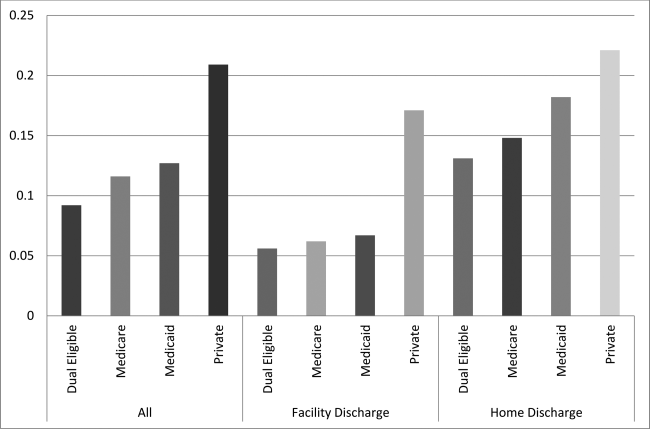
SCHOLAR Project
The structure and function of academic hospital medicine programs (AHPs) has evolved significantly with the growth of hospital medicine.[1, 2, 3, 4] Many AHPs formed in response to regulatory and financial changes, which drove demand for increased trainee oversight, improved clinical efficiency, and growth in nonteaching services staffed by hospitalists. Differences in local organizational contexts and needs have contributed to great variability in AHP program design and operations. As AHPs have become more established, the need to engage academic hospitalists in scholarship and activities that support professional development and promotion has been recognized. Defining sustainable and successful positions for academic hospitalists is a priority called for by leaders in the field.[5, 6]
In this rapidly evolving context, AHPs have employed a variety of approaches to organizing clinical and academic faculty roles, without guiding evidence or consensus‐based performance benchmarks. A number of AHPs have achieved success along traditional academic metrics of research, scholarship, and education. Currently, it is not known whether specific approaches to AHP organization, structure, or definition of faculty roles are associated with achievement of more traditional markers of academic success.
The Academic Committee of the Society of Hospital Medicine (SHM), and the Academic Hospitalist Task Force of the Society of General Internal Medicine (SGIM) had separately initiated projects to explore characteristics associated with success in AHPs. In 2012, these organizations combined efforts to jointly develop and implement the SCHOLAR (SuCcessful HOspitaLists in Academics and Research) project. The goals were to identify successful AHPs using objective criteria, and to then study those groups in greater detail to generate insights that would be broadly relevant to the field. Efforts to clarify the factors within AHPs linked to success by traditional academic metrics will benefit hospitalists, their leaders, and key stakeholders striving to achieve optimal balance between clinical and academic roles. We describe the initial work of the SCHOLAR project, our definitions of academic success in AHPs, and the characteristics of a cohort of exemplary AHPs who achieved the highest levels on these metrics.
METHODS
Defining Success
The 11 members of the SCHOLAR project held a variety of clinical and academic roles within a geographically diverse group of AHPs. We sought to create a functional definition of success applicable to AHPs. As no gold standard currently exists, we used a consensus process among task force members to arrive at a definition that was quantifiable, feasible, and meaningful. The first step was brainstorming on conference calls held 1 to 2 times monthly over 4 months. Potential defining characteristics that emerged from these discussions related to research, teaching, and administrative activities. When potential characteristics were proposed, we considered how to operationalize each one. Each characteristic was discussed until there was consensus from the entire group. Those around education and administration were the most complex, as many roles are locally driven and defined, and challenging to quantify. For this reason, we focused on promotion as a more global approach to assessing academic hospitalist success in these areas. Although criteria for academic advancement also vary across institutions, we felt that promotion generally reflected having met some threshold of academic success. We also wanted to recognize that scholarship occurs outside the context of funded research. Ultimately, 3 key domains emerged: research grant funding, faculty promotion, and scholarship.
After these 3 domains were identified, the group sought to define quantitative metrics to assess performance. These discussions occurred on subsequent calls over a 4‐month period. Between calls, group members gathered additional information to facilitate assessment of the feasibility of proposed metrics, reporting on progress via email. Again, group consensus was sought for each metric considered. Data on grant funding and successful promotions were available from a previous survey conducted through the SHM in 2011. Leaders from 170 AHPs were contacted, with 50 providing complete responses to the 21‐item questionnaire (see Supporting Information, Appendix 1, in the online version of this article). Results of the survey, heretofore referred to as the Leaders of Academic Hospitalist Programs survey (LAHP‐50), have been described elsewhere.[7] For the purposes of this study, we used the self‐reported data about grant funding and promotions contained in the survey to reflect the current state of the field. Although the survey response rate was approximately 30%, the survey was not anonymous, and many reputationally prominent academic hospitalist programs were represented. For these reasons, the group members felt that the survey results were relevant for the purposes of assessing academic success.
In the LAHP‐50, funding was defined as principal investigator or coinvestigator roles on federally and nonfederally funded research, clinical trials, internal grants, and any other extramurally funded projects. Mean and median funding for the overall sample was calculated. Through a separate question, each program's total faculty full‐time equivalent (FTE) count was reported, allowing us to adjust for group size by assessing both total funding per group and funding/FTE for each responding AHP.
Promotions were defined by the self‐reported number of faculty at each of the following ranks: instructor, assistant professor, associate professor, full professor, and professor above scale/emeritus. In addition, a category of nonacademic track (eg, adjunct faculty, clinical associate) was included to capture hospitalists that did not fit into the traditional promotions categories. We did not distinguish between tenure‐track and nontenure‐track academic ranks. LAHP‐50 survey respondents reported the number of faculty in their group at each academic rank. Given that the majority of academic hospitalists hold a rank of assistant professor or lower,[6, 8, 9] and that the number of full professors was only 3% in the LAHP‐50 cohort, we combined the faculty at the associate and full professor ranks, defining successfully promoted faculty as the percent of hospitalists above the rank of assistant professor.
We created a new metric to assess scholarly output. We had considerable discussion of ways to assess the numbers of peer‐reviewed manuscripts generated by AHPs. However, the group had concerns about the feasibility of identification and attribution of authors to specific AHPs through literature searches. We considered examining only publications in the Journal of Hospital Medicine and the Journal of General Internal Medicine, but felt that this would exclude significant work published by hospitalists in fields of medical education or health services research that would more likely appear in alternate journals. Instead, we quantified scholarship based on the number of abstracts presented at national meetings. We focused on meetings of the SHM and SGIM as the primary professional societies representing hospital medicine. The group felt that even work published outside of the journals of our professional societies would likely be presented at those meetings. We used the following strategy: We reviewed research abstracts accepted for presentation as posters or oral abstracts at the 2010 and 2011 SHM national meetings, and research abstracts with a primary or secondary category of hospital medicine at the 2010 and 2011 SGIM national meetings. By including submissions at both SGIM and SHM meetings, we accounted for the fact that some programs may gravitate more to one society meeting or another. We did not include abstracts in the clinical vignettes or innovations categories. We tallied the number of abstracts by group affiliation of the authors for each of the 4 meetings above and created a cumulative total per group for the 2‐year period. Abstracts with authors from different AHPs were counted once for each individual group. Members of the study group reviewed abstracts from each of the meetings in pairs. Reviewers worked separately and compared tallies of results to ensure consistent tabulations. Internet searches were conducted to identify or confirm author affiliations if it was not apparent in the abstract author list. Abstract tallies were compiled without regard to whether programs had completed the LAHP‐50 survey; thus, we collected data on programs that did not respond to the LAHP‐50 survey.
Identification of the SCHOLAR Cohort
To identify our cohort of top‐performing AHPs, we combined the funding and promotions data from the LAHP‐50 sample with the abstract data. We limited our sample to adult hospital medicine groups to reduce heterogeneity. We created rank lists of programs in each category (grant funding, successful promotions, and scholarship), using data from the LAHP‐50 survey to rank programs on funding and promotions, and data from our abstract counts to rank on scholarship. We limited the top‐performing list in each category to 10 institutions as a cutoff. Because we set a threshold of at least $1 million in total funding, we identified only 9 top performing AHPs with regard to grant funding. We also calculated mean funding/FTE. We chose to rank programs only by funding/FTE rather than total funding per program to better account for group size. For successful promotions, we ranked programs by the percentage of senior faculty. For abstract counts, we included programs whose faculty presented abstracts at a minimum of 2 separate meetings, and ranked programs based on the total number of abstracts per group.
This process resulted in separate lists of top performing programs in each of the 3 domains we associated with academic success, arranged in descending order by grant dollars/FTE, percent of senior faculty, and abstract counts (Table 1). Seventeen different programs were represented across these 3 top 10 lists. One program appeared on all 3 lists, 8 programs appeared on 2 lists, and the remainder appeared on a single list (Table 2). Seven of these programs were identified solely based on abstract presentations, diversifying our top groups beyond only those who completed the LAHP‐50 survey. We considered all of these programs to represent high performance in academic hospital medicine. The group selected this inclusive approach because we recognized that any 1 metric was potentially limited, and we sought to identify diverse pathways to success.
| Funding | Promotions | Scholarship | |
|---|---|---|---|
| Grant $/FTE | Total Grant $ | Senior Faculty, No. (%) | Total Abstract Count |
| |||
| $1,409,090 | $15,500,000 | 3 (60%) | 23 |
| $1,000,000 | $9,000,000 | 3 (60%) | 21 |
| $750,000 | $8,000,000 | 4 (57%) | 20 |
| $478,609 | $6,700,535 | 9 (53%) | 15 |
| $347,826 | $3,000,000 | 8 (44%) | 11 |
| $86,956 | $3,000,000 | 14 (41%) | 11 |
| $66,666 | $2,000,000 | 17 (36%) | 10 |
| $46,153 | $1,500,000 | 9 (33%) | 10 |
| $38,461 | $1,000,000 | 2 (33%) | 9 |
| 4 (31%) | 9 | ||
| Selection Criteria for SCHOLAR Cohort | No. of Programs |
|---|---|
| |
| Abstracts, funding, and promotions | 1 |
| Abstracts plus promotions | 4 |
| Abstracts plus funding | 3 |
| Funding plus promotion | 1 |
| Funding only | 1 |
| Abstract only | 7 |
| Total | 17 |
| Top 10 abstract count | |
| 4 meetings | 2 |
| 3 meetings | 2 |
| 2 meetings | 6 |
The 17 unique adult AHPs appearing on at least 1 of the top 10 lists comprised the SCHOLAR cohort of programs that we studied in greater detail. Data reflecting program demographics were solicited directly from leaders of the AHPs identified in the SCHOLAR cohort, including size and age of program, reporting structure, number of faculty at various academic ranks (for programs that did not complete the LAHP‐50 survey), and number of faculty with fellowship training (defined as any postresidency fellowship program).
Subsequently, we performed comparative analyses between the programs in the SCHOLAR cohort to the general population of AHPs reflected by the LAHP‐50 sample. Because abstract presentations were not recorded in the original LAHP‐50 survey instrument, it was not possible to perform a benchmarking comparison for the scholarship domain.
Data Analysis
To measure the success of the SCHOLAR cohort we compared the grant funding and proportion of successfully promoted faculty at the SCHOLAR programs to those in the overall LAHP‐50 sample. Differences in mean and median grant funding were compared using t tests and Mann‐Whitney rank sum tests. Proportion of promoted faculty were compared using 2 tests. A 2‐tailed of 0.05 was used to test significance of differences.
RESULTS
Demographics
Among the AHPs in the SCHOLAR cohort, the mean program age was 13.2 years (range, 618 years), and the mean program size was 36 faculty (range, 1895; median, 28). On average, 15% of faculty members at SCHOLAR programs were fellowship trained (range, 0%37%). Reporting structure among the SCHOLAR programs was as follows: 53% were an independent division or section of the department of medicine; 29% were a section within general internal medicine, and 18% were an independent clinical group.
Grant Funding
Table 3 compares grant funding in the SCHOLAR programs to programs in the overall LAHP‐50 sample. Mean funding per group and mean funding per FTE were significantly higher in the SCHOLAR group than in the overall sample.
| Funding (Millions) | ||
|---|---|---|
| LAHP‐50 Overall Sample | SCHOLAR | |
| ||
| Median grant funding/AHP | 0.060 | 1.500* |
| Mean grant funding/AHP | 1.147 (015) | 3.984* (015) |
| Median grant funding/FTE | 0.004 | 0.038* |
| Mean grant funding/FTE | 0.095 (01.4) | 0.364* (01.4) |
Thirteen of the SCHOLAR programs were represented in the initial LAHP‐50, but 2 did not report a dollar amount for grants and contracts. Therefore, data for total grant funding were available for only 65% (11 of 17) of the programs in the SCHOLAR cohort. Of note, 28% of AHPs in the overall LAHP‐50 sample reported no external funding sources.
Faculty Promotion
Figure 1 demonstrates the proportion of faculty at various academic ranks. The percent of faculty above the rank of assistant professor in the SCHOLAR programs exceeded those in the overall LAHP‐50 by 5% (17.9% vs 12.8%, P = 0.01). Of note, 6% of the hospitalists at AHPs in the SCHOLAR programs were on nonfaculty tracks.
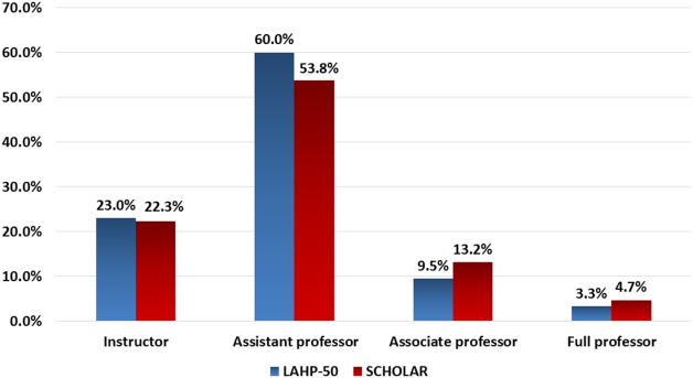
Scholarship
Mean abstract output over the 2‐year period measured was 10.8 (range, 323) in the SCHOLAR cohort. Because we did not collect these data for the LAHP‐50 group, comparative analyses were not possible.
DISCUSSION
Using a definition of academic success that incorporated metrics of grant funding, faculty promotion, and scholarly output, we identified a unique subset of successful AHPsthe SCHOLAR cohort. The programs represented in the SCHOLAR cohort were generally large and relatively mature. Despite this, the cohort consisted of mostly junior faculty, had a paucity of fellowship‐trained hospitalists, and not all reported grant funding.
Prior published work reported complementary findings.[6, 8, 9] A survey of 20 large, well‐established academic hospitalist programs in 2008 found that the majority of hospitalists were junior faculty with a limited publication portfolio. Of the 266 respondents in that study, 86% reported an academic rank at or below assistant professor; funding was not explored.[9] Our similar findings 4 years later add to this work by demonstrating trends over time, and suggest that progress toward creating successful pathways for academic advancement has been slow. In a 2012 survey of the SHM membership, 28% of hospitalists with academic appointments reported no current or future plans to engage in research.[8] These findings suggest that faculty in AHPs may define scholarship through nontraditional pathways, or in some cases choose not to pursue or prioritize scholarship altogether.
Our findings also add to the literature with regard to our assessment of funding, which was variable across the SCHOLAR group. The broad range of funding in the SCHOLAR programs for which we have data (grant dollars $0$15 million per program) suggests that opportunities to improve supported scholarship remain, even among a selected cohort of successful AHPs. The predominance of junior faculty in the SCHOLAR programs may be a reason for this variation. Junior faculty may be engaged in research with funding directed to senior mentors outside their AHP. Alternatively, they may pursue meaningful local hospital quality improvement or educational innovations not supported by external grants, or hold leadership roles in education, quality, or information technology that allow for advancement and promotion without external grant funding. As the scope and impact of these roles increases, senior leaders with alternate sources of support may rely less on research funds; this too may explain some of the differences. Our findings are congruent with results of a study that reviewed original research published by hospitalists, and concluded that the majority of hospitalist research was not externally funded.[8] Our approach for assessing grant funding by adjusting for FTE had the potential to inadvertently favor smaller well‐funded groups over larger ones; however, programs in our sample were similarly represented when ranked by funding/FTE or total grant dollars. As many successful AHPs do concentrate their research funding among a core of focused hospitalist researchers, our definition may not be the ideal metric for some programs.
We chose to define scholarship based on abstract output, rather than peer‐reviewed publications. Although this choice was necessary from a feasibility perspective, it may have excluded programs that prioritize peer‐reviewed publications over abstracts. Although we were unable to incorporate a search strategy to accurately and comprehensively track the publication output attributed specifically to hospitalist researchers and quantify it by program, others have since defined such an approach.[8] However, tracking abstracts theoretically allowed insights into a larger volume of innovative and creative work generated by top AHPs by potentially including work in the earlier stages of development.
We used a consensus‐based definition of success to define our SCHOLAR cohort. There are other ways to measure academic success, which if applied, may have yielded a different sample of programs. For example, over half of the original research articles published in the Journal of Hospital Medicine over a 7‐year span were generated from 5 academic centers.[8] This definition of success may be equally credible, though we note that 4 of these 5 programs were also included in the SCHOLAR cohort. We feel our broader approach was more reflective of the variety of pathways to success available to academic hospitalists. Before our metrics are applied as a benchmarking tool, however, they should ideally be combined with factors not measured in our study to ensure a more comprehensive or balanced reflection of academic success. Factors such as mentorship, level of hospitalist engagement,[10] prevalence of leadership opportunities, operational and fiscal infrastructure, and the impact of local quality, safety, and value efforts should be considered.
Comparison of successfully promoted faculty at AHPs across the country is inherently limited by the wide variation in promotion standards across different institutions; controlling for such differences was not possible with our methodology. For example, it appears that several programs with relatively few senior faculty may have met metrics leading to their inclusion in the SCHOLAR group because of their small program size. Future benchmarking efforts for promotion at AHPs should take scaling into account and consider both total number as well as percentage of senior faculty when evaluating success.
Our methodology has several limitations. Survey data were self‐reported and not independently validated, and as such are subject to recall and reporting biases. Response bias inherently excluded some AHPs that may have met our grant funding or promotions criteria had they participated in the initial LAHP‐50 survey, though we identified and included additional programs through our scholarship metric, increasing the representativeness of the SCHOLAR cohort. Given the dynamic nature of the field, the age of the data we relied upon for analysis limits the generalizability of our specific benchmarks to current practice. However, the development of academic success occurs over the long‐term, and published data on academic hospitalist productivity are consistent with this slower time course.[8] Despite these limitations, our data inform the general topic of gauging performance of AHPs, underscoring the challenges of developing and applying metrics of success, and highlight the variability of performance on selected metrics even among a relatively small group of 17 programs.
In conclusion, we have created a method to quantify academic success that may be useful to academic hospitalists and their group leaders as they set targets for improvement in the field. Even among our SCHOLAR cohort, room for ongoing improvement in development of funded scholarship and a core of senior faculty exists. Further investigation into the unique features of successful groups will offer insight to leaders in academic hospital medicine regarding infrastructure and processes that should be embraced to raise the bar for all AHPs. In addition, efforts to further define and validate nontraditional approaches to scholarship that allow for successful promotion at AHPs would be informative. We view our work less as a singular approach to benchmarking standards for AHPs, and more a call to action to continue efforts to balance scholarly activity and broad professional development of academic hospitalists with increasing clinical demands.
Acknowledgements
The authors thank all of the AHP leaders who participated in the SCHOLAR project. They also thank the Society of Hospital Medicine and Society of General Internal Medicine and the SHM Academic Committee and SGIM Academic Hospitalist Task Force for their support of this work.
Disclosures
The work reported here was supported by the Department of Veterans Affairs, Veterans Health Administration, South Texas Veterans Health Care System. The views expressed in this article are those of the authors and do not necessarily reflect the position or policy of the Department of Veterans Affairs. The authors report no conflicts of interest.
- , , , , . Characteristics of primary care providers who adopted the hospitalist model from 2001 to 2009. J Hosp Med. 2015;10(2):75–82.
- , , , . Growth in the care of older patients by hospitalists in the United States. N Engl J Med. 2009;360(11):1102–1112.
- , , , , . Updating threshold‐based identification of hospitalists in 2012 Medicare pay data. J Hosp Med. 2016;11(1):45–47.
- , , , . Use of hospitalists by Medicare beneficiaries: a national picture. Medicare Medicaid Res Rev. 2014;4(2).
- , , , , , . Challenges and opportunities in Academic Hospital Medicine: report from the Academic Hospital Medicine Summit. J Hosp Med. 2009;4(4):240–246.
- , , , . Survey of US academic hospitalist leaders about mentorship and academic activities in hospitalist groups. J Hosp Med. 2011;6(1):5–9.
- , , , , , . The structure of hospital medicine programs at academic medical centers [abstract]. J Hosp Med. 2012;7(suppl 2):s92.
- , , , , . Research and publication trends in hospital medicine. J Hosp Med. 2014;9(3):148–154.
- , , , , , . Mentorship, productivity, and promotion among academic hospitalists. J Gen Intern Med. 2012;27(1):23–27.
- , , , et al. The key principles and characteristics of an effective hospital medicine group: an assessment guide for hospitals and hospitalists. J Hosp Med. 2014;9(2):123–128.
The structure and function of academic hospital medicine programs (AHPs) has evolved significantly with the growth of hospital medicine.[1, 2, 3, 4] Many AHPs formed in response to regulatory and financial changes, which drove demand for increased trainee oversight, improved clinical efficiency, and growth in nonteaching services staffed by hospitalists. Differences in local organizational contexts and needs have contributed to great variability in AHP program design and operations. As AHPs have become more established, the need to engage academic hospitalists in scholarship and activities that support professional development and promotion has been recognized. Defining sustainable and successful positions for academic hospitalists is a priority called for by leaders in the field.[5, 6]
In this rapidly evolving context, AHPs have employed a variety of approaches to organizing clinical and academic faculty roles, without guiding evidence or consensus‐based performance benchmarks. A number of AHPs have achieved success along traditional academic metrics of research, scholarship, and education. Currently, it is not known whether specific approaches to AHP organization, structure, or definition of faculty roles are associated with achievement of more traditional markers of academic success.
The Academic Committee of the Society of Hospital Medicine (SHM), and the Academic Hospitalist Task Force of the Society of General Internal Medicine (SGIM) had separately initiated projects to explore characteristics associated with success in AHPs. In 2012, these organizations combined efforts to jointly develop and implement the SCHOLAR (SuCcessful HOspitaLists in Academics and Research) project. The goals were to identify successful AHPs using objective criteria, and to then study those groups in greater detail to generate insights that would be broadly relevant to the field. Efforts to clarify the factors within AHPs linked to success by traditional academic metrics will benefit hospitalists, their leaders, and key stakeholders striving to achieve optimal balance between clinical and academic roles. We describe the initial work of the SCHOLAR project, our definitions of academic success in AHPs, and the characteristics of a cohort of exemplary AHPs who achieved the highest levels on these metrics.
METHODS
Defining Success
The 11 members of the SCHOLAR project held a variety of clinical and academic roles within a geographically diverse group of AHPs. We sought to create a functional definition of success applicable to AHPs. As no gold standard currently exists, we used a consensus process among task force members to arrive at a definition that was quantifiable, feasible, and meaningful. The first step was brainstorming on conference calls held 1 to 2 times monthly over 4 months. Potential defining characteristics that emerged from these discussions related to research, teaching, and administrative activities. When potential characteristics were proposed, we considered how to operationalize each one. Each characteristic was discussed until there was consensus from the entire group. Those around education and administration were the most complex, as many roles are locally driven and defined, and challenging to quantify. For this reason, we focused on promotion as a more global approach to assessing academic hospitalist success in these areas. Although criteria for academic advancement also vary across institutions, we felt that promotion generally reflected having met some threshold of academic success. We also wanted to recognize that scholarship occurs outside the context of funded research. Ultimately, 3 key domains emerged: research grant funding, faculty promotion, and scholarship.
After these 3 domains were identified, the group sought to define quantitative metrics to assess performance. These discussions occurred on subsequent calls over a 4‐month period. Between calls, group members gathered additional information to facilitate assessment of the feasibility of proposed metrics, reporting on progress via email. Again, group consensus was sought for each metric considered. Data on grant funding and successful promotions were available from a previous survey conducted through the SHM in 2011. Leaders from 170 AHPs were contacted, with 50 providing complete responses to the 21‐item questionnaire (see Supporting Information, Appendix 1, in the online version of this article). Results of the survey, heretofore referred to as the Leaders of Academic Hospitalist Programs survey (LAHP‐50), have been described elsewhere.[7] For the purposes of this study, we used the self‐reported data about grant funding and promotions contained in the survey to reflect the current state of the field. Although the survey response rate was approximately 30%, the survey was not anonymous, and many reputationally prominent academic hospitalist programs were represented. For these reasons, the group members felt that the survey results were relevant for the purposes of assessing academic success.
In the LAHP‐50, funding was defined as principal investigator or coinvestigator roles on federally and nonfederally funded research, clinical trials, internal grants, and any other extramurally funded projects. Mean and median funding for the overall sample was calculated. Through a separate question, each program's total faculty full‐time equivalent (FTE) count was reported, allowing us to adjust for group size by assessing both total funding per group and funding/FTE for each responding AHP.
Promotions were defined by the self‐reported number of faculty at each of the following ranks: instructor, assistant professor, associate professor, full professor, and professor above scale/emeritus. In addition, a category of nonacademic track (eg, adjunct faculty, clinical associate) was included to capture hospitalists that did not fit into the traditional promotions categories. We did not distinguish between tenure‐track and nontenure‐track academic ranks. LAHP‐50 survey respondents reported the number of faculty in their group at each academic rank. Given that the majority of academic hospitalists hold a rank of assistant professor or lower,[6, 8, 9] and that the number of full professors was only 3% in the LAHP‐50 cohort, we combined the faculty at the associate and full professor ranks, defining successfully promoted faculty as the percent of hospitalists above the rank of assistant professor.
We created a new metric to assess scholarly output. We had considerable discussion of ways to assess the numbers of peer‐reviewed manuscripts generated by AHPs. However, the group had concerns about the feasibility of identification and attribution of authors to specific AHPs through literature searches. We considered examining only publications in the Journal of Hospital Medicine and the Journal of General Internal Medicine, but felt that this would exclude significant work published by hospitalists in fields of medical education or health services research that would more likely appear in alternate journals. Instead, we quantified scholarship based on the number of abstracts presented at national meetings. We focused on meetings of the SHM and SGIM as the primary professional societies representing hospital medicine. The group felt that even work published outside of the journals of our professional societies would likely be presented at those meetings. We used the following strategy: We reviewed research abstracts accepted for presentation as posters or oral abstracts at the 2010 and 2011 SHM national meetings, and research abstracts with a primary or secondary category of hospital medicine at the 2010 and 2011 SGIM national meetings. By including submissions at both SGIM and SHM meetings, we accounted for the fact that some programs may gravitate more to one society meeting or another. We did not include abstracts in the clinical vignettes or innovations categories. We tallied the number of abstracts by group affiliation of the authors for each of the 4 meetings above and created a cumulative total per group for the 2‐year period. Abstracts with authors from different AHPs were counted once for each individual group. Members of the study group reviewed abstracts from each of the meetings in pairs. Reviewers worked separately and compared tallies of results to ensure consistent tabulations. Internet searches were conducted to identify or confirm author affiliations if it was not apparent in the abstract author list. Abstract tallies were compiled without regard to whether programs had completed the LAHP‐50 survey; thus, we collected data on programs that did not respond to the LAHP‐50 survey.
Identification of the SCHOLAR Cohort
To identify our cohort of top‐performing AHPs, we combined the funding and promotions data from the LAHP‐50 sample with the abstract data. We limited our sample to adult hospital medicine groups to reduce heterogeneity. We created rank lists of programs in each category (grant funding, successful promotions, and scholarship), using data from the LAHP‐50 survey to rank programs on funding and promotions, and data from our abstract counts to rank on scholarship. We limited the top‐performing list in each category to 10 institutions as a cutoff. Because we set a threshold of at least $1 million in total funding, we identified only 9 top performing AHPs with regard to grant funding. We also calculated mean funding/FTE. We chose to rank programs only by funding/FTE rather than total funding per program to better account for group size. For successful promotions, we ranked programs by the percentage of senior faculty. For abstract counts, we included programs whose faculty presented abstracts at a minimum of 2 separate meetings, and ranked programs based on the total number of abstracts per group.
This process resulted in separate lists of top performing programs in each of the 3 domains we associated with academic success, arranged in descending order by grant dollars/FTE, percent of senior faculty, and abstract counts (Table 1). Seventeen different programs were represented across these 3 top 10 lists. One program appeared on all 3 lists, 8 programs appeared on 2 lists, and the remainder appeared on a single list (Table 2). Seven of these programs were identified solely based on abstract presentations, diversifying our top groups beyond only those who completed the LAHP‐50 survey. We considered all of these programs to represent high performance in academic hospital medicine. The group selected this inclusive approach because we recognized that any 1 metric was potentially limited, and we sought to identify diverse pathways to success.
| Funding | Promotions | Scholarship | |
|---|---|---|---|
| Grant $/FTE | Total Grant $ | Senior Faculty, No. (%) | Total Abstract Count |
| |||
| $1,409,090 | $15,500,000 | 3 (60%) | 23 |
| $1,000,000 | $9,000,000 | 3 (60%) | 21 |
| $750,000 | $8,000,000 | 4 (57%) | 20 |
| $478,609 | $6,700,535 | 9 (53%) | 15 |
| $347,826 | $3,000,000 | 8 (44%) | 11 |
| $86,956 | $3,000,000 | 14 (41%) | 11 |
| $66,666 | $2,000,000 | 17 (36%) | 10 |
| $46,153 | $1,500,000 | 9 (33%) | 10 |
| $38,461 | $1,000,000 | 2 (33%) | 9 |
| 4 (31%) | 9 | ||
| Selection Criteria for SCHOLAR Cohort | No. of Programs |
|---|---|
| |
| Abstracts, funding, and promotions | 1 |
| Abstracts plus promotions | 4 |
| Abstracts plus funding | 3 |
| Funding plus promotion | 1 |
| Funding only | 1 |
| Abstract only | 7 |
| Total | 17 |
| Top 10 abstract count | |
| 4 meetings | 2 |
| 3 meetings | 2 |
| 2 meetings | 6 |
The 17 unique adult AHPs appearing on at least 1 of the top 10 lists comprised the SCHOLAR cohort of programs that we studied in greater detail. Data reflecting program demographics were solicited directly from leaders of the AHPs identified in the SCHOLAR cohort, including size and age of program, reporting structure, number of faculty at various academic ranks (for programs that did not complete the LAHP‐50 survey), and number of faculty with fellowship training (defined as any postresidency fellowship program).
Subsequently, we performed comparative analyses between the programs in the SCHOLAR cohort to the general population of AHPs reflected by the LAHP‐50 sample. Because abstract presentations were not recorded in the original LAHP‐50 survey instrument, it was not possible to perform a benchmarking comparison for the scholarship domain.
Data Analysis
To measure the success of the SCHOLAR cohort we compared the grant funding and proportion of successfully promoted faculty at the SCHOLAR programs to those in the overall LAHP‐50 sample. Differences in mean and median grant funding were compared using t tests and Mann‐Whitney rank sum tests. Proportion of promoted faculty were compared using 2 tests. A 2‐tailed of 0.05 was used to test significance of differences.
RESULTS
Demographics
Among the AHPs in the SCHOLAR cohort, the mean program age was 13.2 years (range, 618 years), and the mean program size was 36 faculty (range, 1895; median, 28). On average, 15% of faculty members at SCHOLAR programs were fellowship trained (range, 0%37%). Reporting structure among the SCHOLAR programs was as follows: 53% were an independent division or section of the department of medicine; 29% were a section within general internal medicine, and 18% were an independent clinical group.
Grant Funding
Table 3 compares grant funding in the SCHOLAR programs to programs in the overall LAHP‐50 sample. Mean funding per group and mean funding per FTE were significantly higher in the SCHOLAR group than in the overall sample.
| Funding (Millions) | ||
|---|---|---|
| LAHP‐50 Overall Sample | SCHOLAR | |
| ||
| Median grant funding/AHP | 0.060 | 1.500* |
| Mean grant funding/AHP | 1.147 (015) | 3.984* (015) |
| Median grant funding/FTE | 0.004 | 0.038* |
| Mean grant funding/FTE | 0.095 (01.4) | 0.364* (01.4) |
Thirteen of the SCHOLAR programs were represented in the initial LAHP‐50, but 2 did not report a dollar amount for grants and contracts. Therefore, data for total grant funding were available for only 65% (11 of 17) of the programs in the SCHOLAR cohort. Of note, 28% of AHPs in the overall LAHP‐50 sample reported no external funding sources.
Faculty Promotion
Figure 1 demonstrates the proportion of faculty at various academic ranks. The percent of faculty above the rank of assistant professor in the SCHOLAR programs exceeded those in the overall LAHP‐50 by 5% (17.9% vs 12.8%, P = 0.01). Of note, 6% of the hospitalists at AHPs in the SCHOLAR programs were on nonfaculty tracks.
Scholarship
Mean abstract output over the 2‐year period measured was 10.8 (range, 323) in the SCHOLAR cohort. Because we did not collect these data for the LAHP‐50 group, comparative analyses were not possible.
DISCUSSION
Using a definition of academic success that incorporated metrics of grant funding, faculty promotion, and scholarly output, we identified a unique subset of successful AHPsthe SCHOLAR cohort. The programs represented in the SCHOLAR cohort were generally large and relatively mature. Despite this, the cohort consisted of mostly junior faculty, had a paucity of fellowship‐trained hospitalists, and not all reported grant funding.
Prior published work reported complementary findings.[6, 8, 9] A survey of 20 large, well‐established academic hospitalist programs in 2008 found that the majority of hospitalists were junior faculty with a limited publication portfolio. Of the 266 respondents in that study, 86% reported an academic rank at or below assistant professor; funding was not explored.[9] Our similar findings 4 years later add to this work by demonstrating trends over time, and suggest that progress toward creating successful pathways for academic advancement has been slow. In a 2012 survey of the SHM membership, 28% of hospitalists with academic appointments reported no current or future plans to engage in research.[8] These findings suggest that faculty in AHPs may define scholarship through nontraditional pathways, or in some cases choose not to pursue or prioritize scholarship altogether.
Our findings also add to the literature with regard to our assessment of funding, which was variable across the SCHOLAR group. The broad range of funding in the SCHOLAR programs for which we have data (grant dollars $0$15 million per program) suggests that opportunities to improve supported scholarship remain, even among a selected cohort of successful AHPs. The predominance of junior faculty in the SCHOLAR programs may be a reason for this variation. Junior faculty may be engaged in research with funding directed to senior mentors outside their AHP. Alternatively, they may pursue meaningful local hospital quality improvement or educational innovations not supported by external grants, or hold leadership roles in education, quality, or information technology that allow for advancement and promotion without external grant funding. As the scope and impact of these roles increases, senior leaders with alternate sources of support may rely less on research funds; this too may explain some of the differences. Our findings are congruent with results of a study that reviewed original research published by hospitalists, and concluded that the majority of hospitalist research was not externally funded.[8] Our approach for assessing grant funding by adjusting for FTE had the potential to inadvertently favor smaller well‐funded groups over larger ones; however, programs in our sample were similarly represented when ranked by funding/FTE or total grant dollars. As many successful AHPs do concentrate their research funding among a core of focused hospitalist researchers, our definition may not be the ideal metric for some programs.
We chose to define scholarship based on abstract output, rather than peer‐reviewed publications. Although this choice was necessary from a feasibility perspective, it may have excluded programs that prioritize peer‐reviewed publications over abstracts. Although we were unable to incorporate a search strategy to accurately and comprehensively track the publication output attributed specifically to hospitalist researchers and quantify it by program, others have since defined such an approach.[8] However, tracking abstracts theoretically allowed insights into a larger volume of innovative and creative work generated by top AHPs by potentially including work in the earlier stages of development.
We used a consensus‐based definition of success to define our SCHOLAR cohort. There are other ways to measure academic success, which if applied, may have yielded a different sample of programs. For example, over half of the original research articles published in the Journal of Hospital Medicine over a 7‐year span were generated from 5 academic centers.[8] This definition of success may be equally credible, though we note that 4 of these 5 programs were also included in the SCHOLAR cohort. We feel our broader approach was more reflective of the variety of pathways to success available to academic hospitalists. Before our metrics are applied as a benchmarking tool, however, they should ideally be combined with factors not measured in our study to ensure a more comprehensive or balanced reflection of academic success. Factors such as mentorship, level of hospitalist engagement,[10] prevalence of leadership opportunities, operational and fiscal infrastructure, and the impact of local quality, safety, and value efforts should be considered.
Comparison of successfully promoted faculty at AHPs across the country is inherently limited by the wide variation in promotion standards across different institutions; controlling for such differences was not possible with our methodology. For example, it appears that several programs with relatively few senior faculty may have met metrics leading to their inclusion in the SCHOLAR group because of their small program size. Future benchmarking efforts for promotion at AHPs should take scaling into account and consider both total number as well as percentage of senior faculty when evaluating success.
Our methodology has several limitations. Survey data were self‐reported and not independently validated, and as such are subject to recall and reporting biases. Response bias inherently excluded some AHPs that may have met our grant funding or promotions criteria had they participated in the initial LAHP‐50 survey, though we identified and included additional programs through our scholarship metric, increasing the representativeness of the SCHOLAR cohort. Given the dynamic nature of the field, the age of the data we relied upon for analysis limits the generalizability of our specific benchmarks to current practice. However, the development of academic success occurs over the long‐term, and published data on academic hospitalist productivity are consistent with this slower time course.[8] Despite these limitations, our data inform the general topic of gauging performance of AHPs, underscoring the challenges of developing and applying metrics of success, and highlight the variability of performance on selected metrics even among a relatively small group of 17 programs.
In conclusion, we have created a method to quantify academic success that may be useful to academic hospitalists and their group leaders as they set targets for improvement in the field. Even among our SCHOLAR cohort, room for ongoing improvement in development of funded scholarship and a core of senior faculty exists. Further investigation into the unique features of successful groups will offer insight to leaders in academic hospital medicine regarding infrastructure and processes that should be embraced to raise the bar for all AHPs. In addition, efforts to further define and validate nontraditional approaches to scholarship that allow for successful promotion at AHPs would be informative. We view our work less as a singular approach to benchmarking standards for AHPs, and more a call to action to continue efforts to balance scholarly activity and broad professional development of academic hospitalists with increasing clinical demands.
Acknowledgements
The authors thank all of the AHP leaders who participated in the SCHOLAR project. They also thank the Society of Hospital Medicine and Society of General Internal Medicine and the SHM Academic Committee and SGIM Academic Hospitalist Task Force for their support of this work.
Disclosures
The work reported here was supported by the Department of Veterans Affairs, Veterans Health Administration, South Texas Veterans Health Care System. The views expressed in this article are those of the authors and do not necessarily reflect the position or policy of the Department of Veterans Affairs. The authors report no conflicts of interest.
- , , , , . Characteristics of primary care providers who adopted the hospitalist model from 2001 to 2009. J Hosp Med. 2015;10(2):75–82.
- , , , . Growth in the care of older patients by hospitalists in the United States. N Engl J Med. 2009;360(11):1102–1112.
- , , , , . Updating threshold‐based identification of hospitalists in 2012 Medicare pay data. J Hosp Med. 2016;11(1):45–47.
- , , , . Use of hospitalists by Medicare beneficiaries: a national picture. Medicare Medicaid Res Rev. 2014;4(2).
- , , , , , . Challenges and opportunities in Academic Hospital Medicine: report from the Academic Hospital Medicine Summit. J Hosp Med. 2009;4(4):240–246.
- , , , . Survey of US academic hospitalist leaders about mentorship and academic activities in hospitalist groups. J Hosp Med. 2011;6(1):5–9.
- , , , , , . The structure of hospital medicine programs at academic medical centers [abstract]. J Hosp Med. 2012;7(suppl 2):s92.
- , , , , . Research and publication trends in hospital medicine. J Hosp Med. 2014;9(3):148–154.
- , , , , , . Mentorship, productivity, and promotion among academic hospitalists. J Gen Intern Med. 2012;27(1):23–27.
- , , , et al. The key principles and characteristics of an effective hospital medicine group: an assessment guide for hospitals and hospitalists. J Hosp Med. 2014;9(2):123–128.

Use of RUS in the Evaluation of AKI
According to the American College of Radiology Appropriateness Criteria, renal ultrasound (RUS) is the most appropriate imaging examination for evaluating patients with acute kidney injury (AKI), with a rating score of 9, representing the strongest level of recommendation.[1, 2] However, recent studies suggest that RUS may be performed in patients with certain risk factors for ureteral obstruction,[1] which would lead to important reductions in the use of medical imaging. Licurse developed a risk stratification framework to help clinicians identify patients in whom RUS was most likely to be beneficial.[2] The model was built based on clinical predictors that included race, recent exposure to inpatient nephrotoxic medications, history of hydronephrosis, recurrent urinary tract infections, benign prostatic hyperplasia, abdominal or pelvic cancer, neurogenic bladder, single functional kidney, previous pelvic surgery, congestive heart failure, and prerenal AKI. It was found, using a cross‐sectional study design that included derivation and validation samples, that a low‐risk population could be identified based on demographic and clinical risk factors; in this population, the prevalence of hydronephrosis, as well as the rate of hydronephrosis requiring an intervention, was only 1%.
However, due to several study limitations, including that it was performed at a single center,[3] the stratification prediction rule has yet to be adopted broadly. Although at least 1 other study has similarly found that RUS may not be efficacious in patients with no suggestive history and with other more likely causes for renal failure,[1] to the best of our knowledge, no large, external, prospective trial to validate the selective use of RUS in patients with AKI has been reported. Therefore, the aim of this study was to evaluate the accuracy and usefulness of the Licurse renal ultrasonography risk stratification model for hospitalized patients with AKI.
METHODS
Study Setting
The study site was a 793‐bed academic, quaternary care, adult hospital with an affiliated cancer center. The requirement to obtain informed consent was waived by the institutional review board for this Health Insurance Portability and Accountability Actcompliant, prospective cohort study.
Study Population
The study cohort included all adult hospitalized patients who underwent an RUS for the indication of AKI over a 23‐month study period, from January 2013 to November 2014. AKI was defined as having a peak rise in serum creatinine level of at least 0.3 mg/dL from baseline, based on data within the electronic health record (EHR). To ensure that the imaging study was not ordered for the purpose of follow‐up or other reasons, patients who were renal transplant recipients, those who had ureteral stent or nephrostomy in place, patients who were recently diagnosed with hydronephrosis on prior imaging, and women who were pregnant were excluded based on retrospective chart review. In patients with multiple renal ultrasounds during the study period, only the first examination was considered.
Data Collection
We collected patient demographics in the study cohort from the EHR. Imaging data were identified using the radiology information system and computerized physician order entry (CPOE) system. For each eligible patient, we collected relevant clinical attributes including: (1) race, (2) history of hydronephrosis, (3) history of recurrent urinary tract infections, (4) history of benign prostatic hyperplasia, (5) history of abdominal or pelvic cancer, (6) history of neurogenic bladder, (7) history of single functional kidney, (8) history of previous pelvic surgery, (9) recent exposure to inpatient nephrotoxic medications, (10) history of congestive heart failure, and (11) history of prerenal AKI. Information was collected from ordering clinicians at the time of imaging order entry using a computerized data capture tool integrated with the CPOE system. The data capture screen is shown in Supporting Figure 1 in the online version of this article. To validate the accuracy and completeness of this data entry, we manually reviewed objective clinical data from a random sample of 80 medical records for 480 clinical attributes. This number was selected based on a calculation of 80% power, 0.05 , and a 0.1 proportion difference.
Patients received +1 point for the presence/absence of each clinical attribute. The sum of points was used to classify the patient's pretest probability of AKI as low (2), medium (3), or high (>3). Both ordering and interpreting clinicians were blinded to the patient's prediction score.
Each RUS report was manually classified (by an internal medicine attending physician and a radiology trainee) as positive or negative for hydronephrosis, defined as any dilatation of the renal pelvis or the calyces. Subsequent use of urologic intervention was determined by full chart review of the sonographic positive cases. We defined these urologic interventions to include stent placement and nephrostomy tube placement. Only interventions performed during the same hospitalization as the index ultrasound were counted.
Outcomes
Our primary outcome was hydronephrosis (HN) diagnosed on ultrasound. Secondary outcome was hydronephrosis resulting in intervention (HNRI), defined as the need for urologic interventions of stent placement or nephrostomy tube placement.
Statistical Analysis
Analyses were performed using Microsoft Excel 2003 (Microsoft Corp., Redmond, WA) and JMP 10 (SAS Institute, Cary, NC). We used 2 to assess for differences in the rates of HN and HNRI across the 3 pretest probability risk groups. Sensitivity, specificity, negative predictive value, efficiency, and the number needed to screen to find 1 case of HN or HNRI for each risk group were calculated. The high and medium risk groups were merged for the purpose of calculating sensitivity and specificity. Efficiency was defined as the percentage of ultrasounds that could have been avoided based on applying the risk stratification model. We additionally performed a sensitivity analysis to evaluate how different cutoff thresholds for classifying low risk patients would affect the accuracy of the Licurse model. A 2‐tailed P value of 0.05 was defined as statistically significant.
RESULTS
During the 23‐month study period, a total of 961 RUS studies were completed for inpatients with AKI; 778 unique studies met our inclusion criteria (Figure 1).

Based on the manual review of objective clinical data from the random sample of 80 medical records for 480 clinical attributes, overall, there was 90.2% (433/480) concordance rate between the structured data entry and that captured in free text in the clinical notes. There were some variations in the concordance rates for each clinical attribute, ranging from 78.8% (63/80) for exposure to nephrotoxic drugs to 95% for history of congestive heart failure.
On univariate analysis, patients with past medical history of hydronephrosis had a 5‐fold higher likelihood of developing a recurrence of hydronephrosis (45.9% [50/109] vs 8.4% [56/669], P 0.001). Similarly, they also had a 9.5‐fold higher likelihood of requiring urologic interventions related to the hydronephrosis (12.8% [14/109] vs 1.4% [9/669], P 0.001). Having diagnoses predisposing the patient for urinary obstruction (benign prostate hyperplasia, abdominal/pelvic cancer, neurogenic bladder, single functional kidney, and history of pelvic surgery) was correlated with the likelihood of both hydronephrosis and the need for urologic intervention. Of the patients with a diagnosis predisposing the patient for urinary obstructions, 22.1% (59/267) had hydronephrosis on imaging, whereas 9.2% (47/511) of patients without such a diagnosis had hydronephrosis (P 0.001).
Conversely, having a recent exposure to nephrotoxic medications was negatively correlated with the likelihood of both hydronephrosis and the need for urologic intervention. Of the patients with recent exposure to nephrotoxic medications, 7.1% (20/280) had hydronephrosis on imaging, whereas the prevalence of hydronephrosis was 17.3% (86/498) in patients without such an exposure (P 0.001) (Table 1).
| Patient Characteristic | With HN, n = 106 | Without HN, n = 672 | P Value |
|---|---|---|---|
| |||
| Demographics | |||
| Age, y, mean SD | 60.5 17.1 | 64.1 16.0 | 0.035* |
| Nonblack | 97 (91.5) | 573 (85.3) | 0.084 |
| Male | 59 (55.7) | 368 (54.8) | 0.863 |
| Past medical history | |||
| Hydronephrosis | 50 (47.2) | 59 (8.8) | 0.001* |
| Recurrent urinary tract infections | 22 (20.75) | 101 (15.0) | 0.133 |
| Congestive heart failure | 9 (5.5) | 155 (23.1) | 0.001* |
| Prerenal status | 36 (34.0) | 272 (40.5) | 0.203 |
| Exposure to nephrotoxic medication | 20 (18.9) | 260 (38.7) | 0.001* |
| Diagnosis consistent with obstruction | 59 (22.1) | 208 (31.0) | 0.001* |
| Benign prostate hyperplasia | 9 (8.5) | 63 (9.4) | 0.770 |
| Abdominal or pelvic cancer | 42 (39.6) | 97 (14.4) | 0.001* |
| Neurogenic bladder | 5 (4.7) | 12 (1.8) | 0.055 |
| Single functional kidney | 6 (18.8) | 26 (81.3) | 0.388 |
| Pelvic surgery | 14 (13.2) | 61 (9.1) | 0.181 |
Adjusted for other covariates, the multiple variable model showed that a diagnosis predisposing patients for obstruction (odds ratio [OR]: 2.0, P = 0.004), history of hydronephrosis (OR: 7.4, P 0.001), absence of a history of congestive heart failure (OR: 2.7, P = 0.009), and lack of exposure to nephrotoxic medications (OR: 1.9, P = 0.022) were statistically significant predictors for hydronephrosis (Table 2).
| Patient Characteristic | Adjusted Odds Ratio (95% Confidence Interval) | P Value |
|---|---|---|
| ||
| Race | ||
| Nonblack (reference = black) | 1.4 (0.73.1) | 0.414 |
| History of recurrent urinary tract infections | ||
| Yes (reference = no) | 0.75 (0.41.3) | 0.346 |
| Diagnosis consistent with possible obstruction* | ||
| Yes (reference = no) | 2.0 (1.23.1) | 0.004 |
| History of HN | ||
| Yes (reference = no) | 7.4 (4.512.3) | 0.001 |
| History of CHF | ||
| No (reference = yes) | 2.7 (1.36.1) | 0.009 |
| History of prerenal AKI, use of pressors, or sepsis | ||
| No (reference = 1) | 1.0 (0.61.7) | 0.846 |
| Exposure to nephrotoxic medications prior to AKI | ||
| No (reference = yes) | 1.9 (1.13.3) | 0.022 |
After applying the Licurse renal ultrasonography risk stratification model, 176 (22.6%), 190 (24.4%), and 412 (53.0%) patients were classified as low risk, medium risk, and high risk for hydronephrosis, respectively. The incidence rates for hydronephrosis in the pretest probability risk groups were 4.0%, 6.8%, and 20.9% for low‐, medium‐, and high‐risk patients, respectively (P 0.0001). The rates for urologic interventions were 1.1%, 0.5%, and 4.9% in the risk groups from low to high (P 0.0001) (Figure 2).
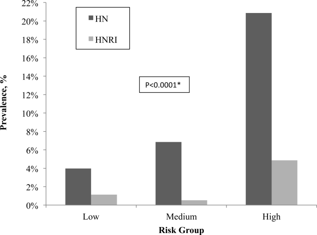
Overall, the Licurse model, using a cutoff between low‐risk and medium/high‐risk patients, had sensitivity of 91.3% (95% confidence interval [CI]: 73.2%‐97.6%) for HNRI and 93.4% (95% CI: 87.0%‐96.8%) for presence of HN. Specificity was low for both HNRI (23.0% [95% CI: 20.2%‐26.2%]) and HN (25.1% [95% CI: 22.0%‐28.6%]). The estimated potential reduction in renal ultrasound for hospitalized patients with AKI, defined as the rate of imaging performed in the low‐risk group, was 22.6%. In the low‐risk group, the number needed to screen to find 1 case of HN was 25, and to find 1 case of HNRI it was 88. The negative predictive value for hydronephrosis was 96.0% (95% CI: 92.0%‐98.1%) and 98.9% for HNRI (95% CI: 96.0%‐99.7%) (Table 3).
| Our External Validation Set | Licurse Internal Validation Set | |||
|---|---|---|---|---|
| HN an Outcome | With HN | Without HN | With HN | Without HN |
| ||||
| Low risk, no. of patients* | 7 | 169 | 7 | 216 |
| Medium/high risk, no. of patients | 99 | 503 | 78 | 496 |
| Test performance, % (95% CI) | ||||
| Sensitivity | 93.4 (87.096.8) | 91.8 (89.993.7) | ||
| Specificity | 25.1 (22.028.6) | 30.3 (27.233.5) | ||
| Negative predictive value | 96.0 (92.098.1) | 96.9 (95.798.1) | ||
| HNRI an outcome | ||||
| Low risk, no. of patients | 2 | 174 | 1 | 222 |
| Medium/high risk, no. of patients | 21 | 581 | 26 | 548 |
| Test performance, % (95% CI) | ||||
| Sensitivity | 91.3 (73.297.6) | 96.3 (94.997.6) | ||
| Specificity | 23.0 (20.226.2) | 28.8 (25.732.0) | ||
| Negative predictive value | 98.9 (96.099.7) | 99.6 (99.1100.0) | ||
Supporting Table 1, in the online version of this article, shows a sensitivity analysis using different cutoff thresholds in the Licurse model for classifying low‐risk patients. A lower threshold cutoff (ie, a cutoff of 1) significantly increases the sensitivity (98.1% [95% CI: 93.4%‐99.5%] for HN; 100% [95% CI: 85.7%‐100%]) for HNRI, but at the cost of a lower specificity (7.6% [95% CI: 5.8%‐9.8%] for HN and 7.0% [95% CI: 5.4%‐9.1%] for HNRI). The estimated potential reduction in renal ultrasound for hospitalized patients with AKI would be 6.0%, the number needed to screen to find 1 case of HN would be 26, and 1 case of HNRI would be infinity.
DISCUSSION
In this prospective observational study, we found that the Licurse risk stratification model, using a cutoff between low‐ risk and medium/high‐risk patients, had 91.3% (95% CI: 73.2%‐97.6%) sensitivity for predicting patients who would require urologic intervention and 93.4% (95% CI: 87.0%‐96.8%) sensitivity for identifying patients with hydronephrosis. These findings were comparable to those found in the original validation cohort of the model, which showed sensitivity rates of 96.3% and 91.8%, respectively.[2] The negative predictive value for hydronephrosis and HNRI were sufficiently high, at 96.0% (95% CI: 92.0‐98.1) and 98.9% (95% CI: 96.0‐99.7), respectively.
Our results suggest that the Licurse model may be sufficient to rule out HN in the inpatient setting at our institution. The slight differences between the findings of our and the original studies may be due to differences in data extraction methodologies. In the original study, all data were retrospectively abstracted from medical records (discharge summaries and clinical notes) by 4 trained reviewers. However, such methodology is dependent on the quality of unstructured EHR data, which as noted in previous research, can be highly variable. Hogan and Wagner found that the correctness of EHR data can range from 44% to 100% and completeness from 1.1% to 100%, depending on the clinical concepts being studied.[4] Similarly, Thiru et al. found that the sensitivity of different types of EHR data ranged from 0.25 to 1.0.[5] Medical chart review can be labor intensive and time consuming. The lack of standardized methods for structured data capture has been a major limitation in decreasing research costs and speeding the rate of new medical discoveries through the secondary use of EHR data. By modifying our institutional clinical decision support (CDS) system to enable the necessary granular clinical data collection, we were able to obviate the need for resource intensive retrospective chart reviews. To our knowledge, this is the second example of a CDS tool specifically designed for capture of discrete data to validate a decision rule.[6] A similar process may also be useful to accelerate generation of new decision rules. With secondary use of EHR data becoming an increasingly important topic,[7] CDS may serve as an alternative method in the context of data reuse for clinical research. Based on a randomly selected chart review, it was noted that clinicians, overall, do try to communicate to the interpreting radiologists the clinical picture as accurately as they can, and rarely do providers drop their orders due to data entry.
Despite our data confirming Licurse's initial findings, it is important to note that as with any clinical prediction rules, there is a trade‐off between cost savings and potential missed diagnoses. Even the most accepted clinical decision rules, such as the Well's criteria for pulmonary embolism and deep vein thrombosis, has their inherent acceptable rates of false negative. What is considered to be acceptable may differ among providers and patients. Thus, a shared decision‐making model, in which the patient and provider actively engage in sharing of information regarding risks and benefits of both performing and bypassing the diagnostic testing, is preferred. For providers/patients who are more risk‐adverse, one could consider using a more sensitive cutoff (for example, using the 1 threshold), essentially increasing the sensitivity from 91.3% to 100% for HNRI and from 93.4% to 98.1% for HN.
Although one would not want to miss a hydronephrosis in a patient, a too aggressive imaging strategy is not without economic and downstream risks. At an estimated cost of $200 per renal ultrasonography,[2] a 22.6% reduction would result in an annual savings of nearly $20,000 at our institution. The financial costs of forgoing ultrasound studies at the risk of missing 1 case of HN or 1 case of HNRI would be $5000 and $17,600, respectively.
Data‐driven decision rules are becoming more commonly used in the current environment of increased emphasis on evidence‐based medicine.[8, 9, 10, 11, 12, 13] When applied appropriately, such prediction models can result in more efficient use of medical imaging while increasing value of care.[14, 15] However, prior to implementation in clinical practice, these models need to be externally validated across multiple institutions and in various practice settings. This is the largest study of which we are aware to validate the utility of a prediction model for AKI in the inpatient setting. Although we did find slightly smaller differences in hydronephrosis in inpatients across the low, moderate, and high pretest probability groups, this may be explained by the differences in methodology.
Our study has several limitations. First, it was performed at a single academic medical center, a similar setting as that of the original work. Thus, the generalizability of our findings in other settings is unclear. Second, it is possible that our ordering providers did not thoroughly and accurately enter data into the structured CPOE form. However, we randomly selected a sample for chart review and found 90% concordance between data captured and those in the EHR. Due to selection of our cohort that included only patients with AKI who underwent RUS, it is possible that some patients who were not imaged or imaged with other cross‐sectional modalities were excluded, resulting in differential test ordering bias. Finally, we did not include the potential benefits of RUS in affecting nonsurgical interventions of hydronephrosis (eg, Foley catheter insertion).
CONCLUSION
We found that the Licurse renal ultrasonography risk stratification model was sufficiently accurate in classifying patients at risk for ureteral obstruction among hospitalized patients with AKI.
Acknowledgements
The authors thank Laura E. Peterson, BSN, SM, for her assistance in editing this manuscript.
- , , , , . Renal sonography: can it be used more selectively in the setting of an elevated serum creatinine level? Am J Kidney Dis. 1997;29(3):362–367.
- . Renal ultrasonography in the evaluation of acute kidney injury: developing a Risk stratification framework. Arch Intern Med. 2010;170(21):1900.
- , . Curbing the use of ultrasonography in the diagnosis of acute kidney injury: Penny wise or pound foolish?: comment on “Renal ultrasonography in the evaluation of acute kidney injury.” Arch Intern Med. 2010;170(21):1907–1908.
- , . Accuracy of data in computer‐based patient records. J Am Med Inform Assoc 1997;4(5):342–355.
- , , . Systematic review of scope and quality of electronic patient record data in primary care. BMJ. 2003;326(7398):1070.
- , , , , , . Performance of Wells score for deep vein thrombosis in the inpatient setting. JAMA Intern Med. 2015;175(7):1112–1117.
- , , , , . Public preferences about secondary uses of electronic health information. JAMA Intern Med. 2013;173(19):1798–1806.
- , , , et al. The Canadian CT Head Rule for patients with minor head injury. Lancet. 2001;357(9266):1391–1396.
- , , , et al. Value of assessment of pretest probability of deep‐vein thrombosis in clinical management. Lancet. 1997;350(9094):1795–1798.
- , , , , , . Derivation of the children's head injury algorithm for the prediction of important clinical events decision rule for head injury in children. Arch Dis Child. 2006;91(11):885–891.
- , , , et al. Clinical decision rules to rule out subarachnoid hemorrhage for acute headache. JAMA. 2013;310(12):1248–1255.
- , , , et al. Excluding pulmonary embolism at the bedside without diagnostic imaging: management of patients with suspected pulmonary embolism presenting to the emergency department by using a simple clinical model and d‐dimer. Ann Intern Med. 2001;135(2):98–107.
- , , , et al. Implementation of the Ottawa knee rule for the use of radiography in acute knee injuries. JAMA. 1997;278(23):2075–2079.
- , , , et al. Impact of provider‐led, technology‐enabled radiology management program on imaging. Am J Med. 2013;126(8):687–692.
- , , , et al. Effect of computerized clinical decision support on the use and yield of CT pulmonary angiography in the emergency department. Radiology. 2012;262(2):468–474.
According to the American College of Radiology Appropriateness Criteria, renal ultrasound (RUS) is the most appropriate imaging examination for evaluating patients with acute kidney injury (AKI), with a rating score of 9, representing the strongest level of recommendation.[1, 2] However, recent studies suggest that RUS may be performed in patients with certain risk factors for ureteral obstruction,[1] which would lead to important reductions in the use of medical imaging. Licurse developed a risk stratification framework to help clinicians identify patients in whom RUS was most likely to be beneficial.[2] The model was built based on clinical predictors that included race, recent exposure to inpatient nephrotoxic medications, history of hydronephrosis, recurrent urinary tract infections, benign prostatic hyperplasia, abdominal or pelvic cancer, neurogenic bladder, single functional kidney, previous pelvic surgery, congestive heart failure, and prerenal AKI. It was found, using a cross‐sectional study design that included derivation and validation samples, that a low‐risk population could be identified based on demographic and clinical risk factors; in this population, the prevalence of hydronephrosis, as well as the rate of hydronephrosis requiring an intervention, was only 1%.
However, due to several study limitations, including that it was performed at a single center,[3] the stratification prediction rule has yet to be adopted broadly. Although at least 1 other study has similarly found that RUS may not be efficacious in patients with no suggestive history and with other more likely causes for renal failure,[1] to the best of our knowledge, no large, external, prospective trial to validate the selective use of RUS in patients with AKI has been reported. Therefore, the aim of this study was to evaluate the accuracy and usefulness of the Licurse renal ultrasonography risk stratification model for hospitalized patients with AKI.
METHODS
Study Setting
The study site was a 793‐bed academic, quaternary care, adult hospital with an affiliated cancer center. The requirement to obtain informed consent was waived by the institutional review board for this Health Insurance Portability and Accountability Actcompliant, prospective cohort study.
Study Population
The study cohort included all adult hospitalized patients who underwent an RUS for the indication of AKI over a 23‐month study period, from January 2013 to November 2014. AKI was defined as having a peak rise in serum creatinine level of at least 0.3 mg/dL from baseline, based on data within the electronic health record (EHR). To ensure that the imaging study was not ordered for the purpose of follow‐up or other reasons, patients who were renal transplant recipients, those who had ureteral stent or nephrostomy in place, patients who were recently diagnosed with hydronephrosis on prior imaging, and women who were pregnant were excluded based on retrospective chart review. In patients with multiple renal ultrasounds during the study period, only the first examination was considered.
Data Collection
We collected patient demographics in the study cohort from the EHR. Imaging data were identified using the radiology information system and computerized physician order entry (CPOE) system. For each eligible patient, we collected relevant clinical attributes including: (1) race, (2) history of hydronephrosis, (3) history of recurrent urinary tract infections, (4) history of benign prostatic hyperplasia, (5) history of abdominal or pelvic cancer, (6) history of neurogenic bladder, (7) history of single functional kidney, (8) history of previous pelvic surgery, (9) recent exposure to inpatient nephrotoxic medications, (10) history of congestive heart failure, and (11) history of prerenal AKI. Information was collected from ordering clinicians at the time of imaging order entry using a computerized data capture tool integrated with the CPOE system. The data capture screen is shown in Supporting Figure 1 in the online version of this article. To validate the accuracy and completeness of this data entry, we manually reviewed objective clinical data from a random sample of 80 medical records for 480 clinical attributes. This number was selected based on a calculation of 80% power, 0.05 , and a 0.1 proportion difference.
Patients received +1 point for the presence/absence of each clinical attribute. The sum of points was used to classify the patient's pretest probability of AKI as low (2), medium (3), or high (>3). Both ordering and interpreting clinicians were blinded to the patient's prediction score.
Each RUS report was manually classified (by an internal medicine attending physician and a radiology trainee) as positive or negative for hydronephrosis, defined as any dilatation of the renal pelvis or the calyces. Subsequent use of urologic intervention was determined by full chart review of the sonographic positive cases. We defined these urologic interventions to include stent placement and nephrostomy tube placement. Only interventions performed during the same hospitalization as the index ultrasound were counted.
Outcomes
Our primary outcome was hydronephrosis (HN) diagnosed on ultrasound. Secondary outcome was hydronephrosis resulting in intervention (HNRI), defined as the need for urologic interventions of stent placement or nephrostomy tube placement.
Statistical Analysis
Analyses were performed using Microsoft Excel 2003 (Microsoft Corp., Redmond, WA) and JMP 10 (SAS Institute, Cary, NC). We used 2 to assess for differences in the rates of HN and HNRI across the 3 pretest probability risk groups. Sensitivity, specificity, negative predictive value, efficiency, and the number needed to screen to find 1 case of HN or HNRI for each risk group were calculated. The high and medium risk groups were merged for the purpose of calculating sensitivity and specificity. Efficiency was defined as the percentage of ultrasounds that could have been avoided based on applying the risk stratification model. We additionally performed a sensitivity analysis to evaluate how different cutoff thresholds for classifying low risk patients would affect the accuracy of the Licurse model. A 2‐tailed P value of 0.05 was defined as statistically significant.
RESULTS
During the 23‐month study period, a total of 961 RUS studies were completed for inpatients with AKI; 778 unique studies met our inclusion criteria (Figure 1).
Based on the manual review of objective clinical data from the random sample of 80 medical records for 480 clinical attributes, overall, there was 90.2% (433/480) concordance rate between the structured data entry and that captured in free text in the clinical notes. There were some variations in the concordance rates for each clinical attribute, ranging from 78.8% (63/80) for exposure to nephrotoxic drugs to 95% for history of congestive heart failure.
On univariate analysis, patients with past medical history of hydronephrosis had a 5‐fold higher likelihood of developing a recurrence of hydronephrosis (45.9% [50/109] vs 8.4% [56/669], P 0.001). Similarly, they also had a 9.5‐fold higher likelihood of requiring urologic interventions related to the hydronephrosis (12.8% [14/109] vs 1.4% [9/669], P 0.001). Having diagnoses predisposing the patient for urinary obstruction (benign prostate hyperplasia, abdominal/pelvic cancer, neurogenic bladder, single functional kidney, and history of pelvic surgery) was correlated with the likelihood of both hydronephrosis and the need for urologic intervention. Of the patients with a diagnosis predisposing the patient for urinary obstructions, 22.1% (59/267) had hydronephrosis on imaging, whereas 9.2% (47/511) of patients without such a diagnosis had hydronephrosis (P 0.001).
Conversely, having a recent exposure to nephrotoxic medications was negatively correlated with the likelihood of both hydronephrosis and the need for urologic intervention. Of the patients with recent exposure to nephrotoxic medications, 7.1% (20/280) had hydronephrosis on imaging, whereas the prevalence of hydronephrosis was 17.3% (86/498) in patients without such an exposure (P 0.001) (Table 1).
| Patient Characteristic | With HN, n = 106 | Without HN, n = 672 | P Value |
|---|---|---|---|
| |||
| Demographics | |||
| Age, y, mean SD | 60.5 17.1 | 64.1 16.0 | 0.035* |
| Nonblack | 97 (91.5) | 573 (85.3) | 0.084 |
| Male | 59 (55.7) | 368 (54.8) | 0.863 |
| Past medical history | |||
| Hydronephrosis | 50 (47.2) | 59 (8.8) | 0.001* |
| Recurrent urinary tract infections | 22 (20.75) | 101 (15.0) | 0.133 |
| Congestive heart failure | 9 (5.5) | 155 (23.1) | 0.001* |
| Prerenal status | 36 (34.0) | 272 (40.5) | 0.203 |
| Exposure to nephrotoxic medication | 20 (18.9) | 260 (38.7) | 0.001* |
| Diagnosis consistent with obstruction | 59 (22.1) | 208 (31.0) | 0.001* |
| Benign prostate hyperplasia | 9 (8.5) | 63 (9.4) | 0.770 |
| Abdominal or pelvic cancer | 42 (39.6) | 97 (14.4) | 0.001* |
| Neurogenic bladder | 5 (4.7) | 12 (1.8) | 0.055 |
| Single functional kidney | 6 (18.8) | 26 (81.3) | 0.388 |
| Pelvic surgery | 14 (13.2) | 61 (9.1) | 0.181 |
Adjusted for other covariates, the multiple variable model showed that a diagnosis predisposing patients for obstruction (odds ratio [OR]: 2.0, P = 0.004), history of hydronephrosis (OR: 7.4, P 0.001), absence of a history of congestive heart failure (OR: 2.7, P = 0.009), and lack of exposure to nephrotoxic medications (OR: 1.9, P = 0.022) were statistically significant predictors for hydronephrosis (Table 2).
| Patient Characteristic | Adjusted Odds Ratio (95% Confidence Interval) | P Value |
|---|---|---|
| ||
| Race | ||
| Nonblack (reference = black) | 1.4 (0.73.1) | 0.414 |
| History of recurrent urinary tract infections | ||
| Yes (reference = no) | 0.75 (0.41.3) | 0.346 |
| Diagnosis consistent with possible obstruction* | ||
| Yes (reference = no) | 2.0 (1.23.1) | 0.004 |
| History of HN | ||
| Yes (reference = no) | 7.4 (4.512.3) | 0.001 |
| History of CHF | ||
| No (reference = yes) | 2.7 (1.36.1) | 0.009 |
| History of prerenal AKI, use of pressors, or sepsis | ||
| No (reference = 1) | 1.0 (0.61.7) | 0.846 |
| Exposure to nephrotoxic medications prior to AKI | ||
| No (reference = yes) | 1.9 (1.13.3) | 0.022 |
After applying the Licurse renal ultrasonography risk stratification model, 176 (22.6%), 190 (24.4%), and 412 (53.0%) patients were classified as low risk, medium risk, and high risk for hydronephrosis, respectively. The incidence rates for hydronephrosis in the pretest probability risk groups were 4.0%, 6.8%, and 20.9% for low‐, medium‐, and high‐risk patients, respectively (P 0.0001). The rates for urologic interventions were 1.1%, 0.5%, and 4.9% in the risk groups from low to high (P 0.0001) (Figure 2).
Overall, the Licurse model, using a cutoff between low‐risk and medium/high‐risk patients, had sensitivity of 91.3% (95% confidence interval [CI]: 73.2%‐97.6%) for HNRI and 93.4% (95% CI: 87.0%‐96.8%) for presence of HN. Specificity was low for both HNRI (23.0% [95% CI: 20.2%‐26.2%]) and HN (25.1% [95% CI: 22.0%‐28.6%]). The estimated potential reduction in renal ultrasound for hospitalized patients with AKI, defined as the rate of imaging performed in the low‐risk group, was 22.6%. In the low‐risk group, the number needed to screen to find 1 case of HN was 25, and to find 1 case of HNRI it was 88. The negative predictive value for hydronephrosis was 96.0% (95% CI: 92.0%‐98.1%) and 98.9% for HNRI (95% CI: 96.0%‐99.7%) (Table 3).
| Our External Validation Set | Licurse Internal Validation Set | |||
|---|---|---|---|---|
| HN an Outcome | With HN | Without HN | With HN | Without HN |
| ||||
| Low risk, no. of patients* | 7 | 169 | 7 | 216 |
| Medium/high risk, no. of patients | 99 | 503 | 78 | 496 |
| Test performance, % (95% CI) | ||||
| Sensitivity | 93.4 (87.096.8) | 91.8 (89.993.7) | ||
| Specificity | 25.1 (22.028.6) | 30.3 (27.233.5) | ||
| Negative predictive value | 96.0 (92.098.1) | 96.9 (95.798.1) | ||
| HNRI an outcome | ||||
| Low risk, no. of patients | 2 | 174 | 1 | 222 |
| Medium/high risk, no. of patients | 21 | 581 | 26 | 548 |
| Test performance, % (95% CI) | ||||
| Sensitivity | 91.3 (73.297.6) | 96.3 (94.997.6) | ||
| Specificity | 23.0 (20.226.2) | 28.8 (25.732.0) | ||
| Negative predictive value | 98.9 (96.099.7) | 99.6 (99.1100.0) | ||
Supporting Table 1, in the online version of this article, shows a sensitivity analysis using different cutoff thresholds in the Licurse model for classifying low‐risk patients. A lower threshold cutoff (ie, a cutoff of 1) significantly increases the sensitivity (98.1% [95% CI: 93.4%‐99.5%] for HN; 100% [95% CI: 85.7%‐100%]) for HNRI, but at the cost of a lower specificity (7.6% [95% CI: 5.8%‐9.8%] for HN and 7.0% [95% CI: 5.4%‐9.1%] for HNRI). The estimated potential reduction in renal ultrasound for hospitalized patients with AKI would be 6.0%, the number needed to screen to find 1 case of HN would be 26, and 1 case of HNRI would be infinity.
DISCUSSION
In this prospective observational study, we found that the Licurse risk stratification model, using a cutoff between low‐ risk and medium/high‐risk patients, had 91.3% (95% CI: 73.2%‐97.6%) sensitivity for predicting patients who would require urologic intervention and 93.4% (95% CI: 87.0%‐96.8%) sensitivity for identifying patients with hydronephrosis. These findings were comparable to those found in the original validation cohort of the model, which showed sensitivity rates of 96.3% and 91.8%, respectively.[2] The negative predictive value for hydronephrosis and HNRI were sufficiently high, at 96.0% (95% CI: 92.0‐98.1) and 98.9% (95% CI: 96.0‐99.7), respectively.
Our results suggest that the Licurse model may be sufficient to rule out HN in the inpatient setting at our institution. The slight differences between the findings of our and the original studies may be due to differences in data extraction methodologies. In the original study, all data were retrospectively abstracted from medical records (discharge summaries and clinical notes) by 4 trained reviewers. However, such methodology is dependent on the quality of unstructured EHR data, which as noted in previous research, can be highly variable. Hogan and Wagner found that the correctness of EHR data can range from 44% to 100% and completeness from 1.1% to 100%, depending on the clinical concepts being studied.[4] Similarly, Thiru et al. found that the sensitivity of different types of EHR data ranged from 0.25 to 1.0.[5] Medical chart review can be labor intensive and time consuming. The lack of standardized methods for structured data capture has been a major limitation in decreasing research costs and speeding the rate of new medical discoveries through the secondary use of EHR data. By modifying our institutional clinical decision support (CDS) system to enable the necessary granular clinical data collection, we were able to obviate the need for resource intensive retrospective chart reviews. To our knowledge, this is the second example of a CDS tool specifically designed for capture of discrete data to validate a decision rule.[6] A similar process may also be useful to accelerate generation of new decision rules. With secondary use of EHR data becoming an increasingly important topic,[7] CDS may serve as an alternative method in the context of data reuse for clinical research. Based on a randomly selected chart review, it was noted that clinicians, overall, do try to communicate to the interpreting radiologists the clinical picture as accurately as they can, and rarely do providers drop their orders due to data entry.
Despite our data confirming Licurse's initial findings, it is important to note that as with any clinical prediction rules, there is a trade‐off between cost savings and potential missed diagnoses. Even the most accepted clinical decision rules, such as the Well's criteria for pulmonary embolism and deep vein thrombosis, has their inherent acceptable rates of false negative. What is considered to be acceptable may differ among providers and patients. Thus, a shared decision‐making model, in which the patient and provider actively engage in sharing of information regarding risks and benefits of both performing and bypassing the diagnostic testing, is preferred. For providers/patients who are more risk‐adverse, one could consider using a more sensitive cutoff (for example, using the 1 threshold), essentially increasing the sensitivity from 91.3% to 100% for HNRI and from 93.4% to 98.1% for HN.
Although one would not want to miss a hydronephrosis in a patient, a too aggressive imaging strategy is not without economic and downstream risks. At an estimated cost of $200 per renal ultrasonography,[2] a 22.6% reduction would result in an annual savings of nearly $20,000 at our institution. The financial costs of forgoing ultrasound studies at the risk of missing 1 case of HN or 1 case of HNRI would be $5000 and $17,600, respectively.
Data‐driven decision rules are becoming more commonly used in the current environment of increased emphasis on evidence‐based medicine.[8, 9, 10, 11, 12, 13] When applied appropriately, such prediction models can result in more efficient use of medical imaging while increasing value of care.[14, 15] However, prior to implementation in clinical practice, these models need to be externally validated across multiple institutions and in various practice settings. This is the largest study of which we are aware to validate the utility of a prediction model for AKI in the inpatient setting. Although we did find slightly smaller differences in hydronephrosis in inpatients across the low, moderate, and high pretest probability groups, this may be explained by the differences in methodology.
Our study has several limitations. First, it was performed at a single academic medical center, a similar setting as that of the original work. Thus, the generalizability of our findings in other settings is unclear. Second, it is possible that our ordering providers did not thoroughly and accurately enter data into the structured CPOE form. However, we randomly selected a sample for chart review and found 90% concordance between data captured and those in the EHR. Due to selection of our cohort that included only patients with AKI who underwent RUS, it is possible that some patients who were not imaged or imaged with other cross‐sectional modalities were excluded, resulting in differential test ordering bias. Finally, we did not include the potential benefits of RUS in affecting nonsurgical interventions of hydronephrosis (eg, Foley catheter insertion).
CONCLUSION
We found that the Licurse renal ultrasonography risk stratification model was sufficiently accurate in classifying patients at risk for ureteral obstruction among hospitalized patients with AKI.
Acknowledgements
The authors thank Laura E. Peterson, BSN, SM, for her assistance in editing this manuscript.
- , , , , . Renal sonography: can it be used more selectively in the setting of an elevated serum creatinine level? Am J Kidney Dis. 1997;29(3):362–367.
- . Renal ultrasonography in the evaluation of acute kidney injury: developing a Risk stratification framework. Arch Intern Med. 2010;170(21):1900.
- , . Curbing the use of ultrasonography in the diagnosis of acute kidney injury: Penny wise or pound foolish?: comment on “Renal ultrasonography in the evaluation of acute kidney injury.” Arch Intern Med. 2010;170(21):1907–1908.
- , . Accuracy of data in computer‐based patient records. J Am Med Inform Assoc 1997;4(5):342–355.
- , , . Systematic review of scope and quality of electronic patient record data in primary care. BMJ. 2003;326(7398):1070.
- , , , , , . Performance of Wells score for deep vein thrombosis in the inpatient setting. JAMA Intern Med. 2015;175(7):1112–1117.
- , , , , . Public preferences about secondary uses of electronic health information. JAMA Intern Med. 2013;173(19):1798–1806.
- , , , et al. The Canadian CT Head Rule for patients with minor head injury. Lancet. 2001;357(9266):1391–1396.
- , , , et al. Value of assessment of pretest probability of deep‐vein thrombosis in clinical management. Lancet. 1997;350(9094):1795–1798.
- , , , , , . Derivation of the children's head injury algorithm for the prediction of important clinical events decision rule for head injury in children. Arch Dis Child. 2006;91(11):885–891.
- , , , et al. Clinical decision rules to rule out subarachnoid hemorrhage for acute headache. JAMA. 2013;310(12):1248–1255.
- , , , et al. Excluding pulmonary embolism at the bedside without diagnostic imaging: management of patients with suspected pulmonary embolism presenting to the emergency department by using a simple clinical model and d‐dimer. Ann Intern Med. 2001;135(2):98–107.
- , , , et al. Implementation of the Ottawa knee rule for the use of radiography in acute knee injuries. JAMA. 1997;278(23):2075–2079.
- , , , et al. Impact of provider‐led, technology‐enabled radiology management program on imaging. Am J Med. 2013;126(8):687–692.
- , , , et al. Effect of computerized clinical decision support on the use and yield of CT pulmonary angiography in the emergency department. Radiology. 2012;262(2):468–474.
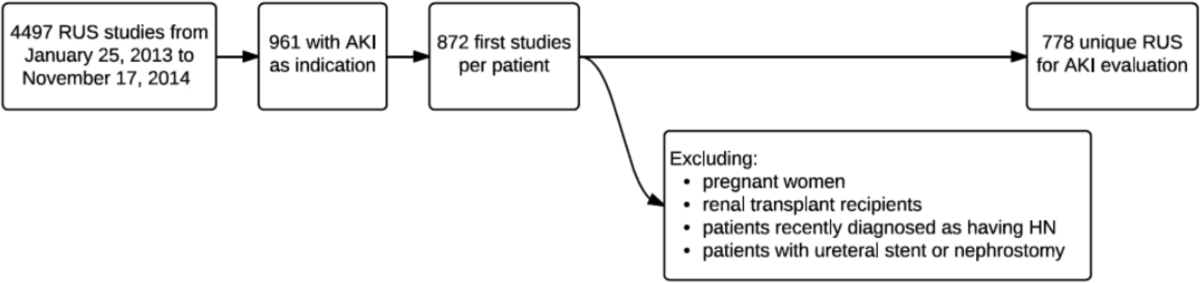
Frailty Evaluation in the Hospital
Frailty is a state of vulnerability that encompasses a heterogeneous group of people.[1] Because it lacks a precise definition, multiple tools have been developed to identify frailty in both clinical and research settings.[2, 3, 4] Prevalence of frailty depends on the frailty assessment tool used and the population studied, ranging from 4% to 17% when the Fried score[5, 6, 7] is used and from 5% to 44%[5, 7, 8] when cumulative deficit models like the Frailty Index are utilized, with the lower prevalences being in younger community‐dwelling elderly populations and the higher proportions being in older institutionalized populations.
The Frailty Index, also called the Burden or Cumulative Deficit Model, comprises 70 domains that include mobility, mood, function, cognitive impairment, and disease states. It is multidimensional and allows for patients to be categorized on a continuum of frailty, but it is extremely difficult to apply in clinical practice. Recognizing this, Rockwood et al.[9] developed and validated the Clinical Frailty Scale (CFS) in the Canadian Study of Health and Aging. The CFS classifies patients into 1 of 9 categories: very fit, well, managing well, vulnerable, mildly frail (needs help with at least 1 instrumental activity of daily living such as shopping, finances, meal preparation, or housework), moderately frail (needs help with 1 or 2 activities of daily living such as bathing and dressing), severely frail (dependent for personal care), very severely frail (bedbound), and terminally ill. Although this tool is easy to use in clinical practice, it reflects a gestalt impression and requires some clinical judgement.
The Fried score[6] is a prototypical phenotype tool based on 5 criteria that include weight loss, self‐reported exhaustion, low energy expenditure, slowness of gait, and weakness. Recent evidence has suggested that slow gait (or dysmobility) alone may also be a potential screening test for frailty.[10] A recent systematic review[11] demonstrated an association between slow gait (dysmobility) and increased mortality. Dysmobility negatively impacts quality of life and has a strong association with disability resulting in the need for an increased level of care.[12] The Timed Up and Go Test (TUGT) is one method of assessing mobility which is relatively easy to perform, does not require special equipment, and is feasible to use in clinical settings.[13] However, whether impaired mobility predicts outcomes within the first 30 days after hospital discharge (a timeframe highlighted in the Affordable Care Act and used by the Centers for Medicare and Medicaid Services as an important hospital quality indicator) is still uncertain.
The aim of this study was to compare frailty assessments using the CFS and 2 of the most commonly used phenotypic tools (a modified Fried score and the TUGT as a proxy for mobility assessment) to determine which tools best predict postdischarge outcomes.
METHODS
Study Design and Population
As described in detail elsewhere,[14] this was a prospective cohort study that enrolled adult patients (any age older than 18 years) at the time of discharge back to the community from 7 general internal medicine wards in 2 teaching hospitals in Edmonton, Alberta between October 2013 and November 2014. We excluded patients admitted from, or being discharged back to, long‐term care facilities or other acute care hospitals, or from out of the province; patients who were unable to communicate in English; patients with moderate or severe cognitive impairment (scoring 5 or more on the Short Portable Mental Status Questionnaire); or patients with projected life expectancy of less than 3 months. All patients provided written consent, and the study was approved by the Health Research Ethics board of the University of Alberta (project ID Pro00036880).
We assessed the degree of frailty within 24 hours of discharge in 3 ways. First, we used the CFS[9, 15] with patients being asked to rate their best functional status in the week prior to admission. As per the CFS validations studies, scores 5 were defined as frail.[9, 15] Second, we used the TUGT as a proxy for slow gait speed/dysmobility (with >20 seconds defined as abnormal).[13] The TUGT was recorded as the shortest recorded time of the 2 timed trials to get up from a seated position, walk 10 feet and back, and then sit in the chair again. Third, we also determined their Fried score[6] (using the modifications outlined below) and categorized the patients as frail if they scored 3 or more. Of the 5 Fried categories, we assessed weakness by grip strength in their dominant hand using a Jamar handheld dynamometer and weight loss of 10 lb or more in the past year based on patient self‐report; these are identical to the original Fried scale description. Grip strength in the lowest quintile for sex and body mass index was defined as weak grip strength as per convention in the literature, which corresponded to less than 28.5 kg for men and less than 18.5 kg for women.[16, 17] We assessed the other 3 Fried categories in modified fashion as follows. For slow gait, rather than assessing time to walk 15 feet as in the original study and assigning a point to those testing in the lowest quintile for their age/sex, we used the TUGT, because our research personnel were already trained in this test, and we were doing it already as part of the discharge package for all patients.[13] For the Fried category of low activity, we based this on patient self‐report using the relevant questions in the EuroQoL Questionnaire (EQ‐5D); the Fried score used self‐report with a different questionnaire. Finally, for self‐reported exhaustion we used the questions in the Patient Health Questionnaire 9 (PHQ‐9)[18] analogous to those used from the Center for Epidemiological Studies depression scale in the original Fried description. We did this as we were evaluating the PHQ‐9 in our cohort already, and did not want to increase responder burden by presenting them with 2 depression questionnaires.
We followed all patients until 30 days after discharge, and outcome data (all‐cause mortality or all‐cause readmission) were collected by research personnel blinded to the patient's frailty status at discharge using patient/caregiver self‐report and analysis of the provincial electronic health record. We included deaths in or out of the hospital, and all readmissions were unplanned.
We examined the correlation between the CFS score (5 vs 5) and (1) the modified Fried score (3 vs 3) and (2) TUGT (20 seconds vs >20 seconds) using chance corrected kappa coefficients. In our previous article[14] we reported the association between the CFS and readmissions/hospitalizations within 30 days of discharge. In this article we examine whether either the Fried score or TUGT accurately and independently predict postdischarge readmissions/deaths, and whether they add additional prognostic information to the CFS assessment by comparing models with/without each definition using the C statistic and the Integrated Discrimination Improvement index. All analyses were performed using SAS version 9.4 (SAS Institute, Cary, NC), with P values of 0.05 considered statistically significant. Subgroup analysis was done in patients older than 65 years.
RESULTS
Of 1124 potentially eligible patients, 626 were excluded because of patient refusal (n = 227); transfer to/from another hospital, long‐term care facility, or out of province (n = 189); moderate to severe cognitive impairment (n = 88); language barriers (n = 71); or foreshortened life expectancy (n = 51). Another 3 patients withdrew consent prior to outcome assessment. The 495 patients we recruited and had outcome data for had a mean age of 64 years, 19.6% were older than 80 years, 50% were women, and the patients had a mean of 4.2 comorbidities and mean Charlson score of 2.4. The 4 most common reasons for hospital admission were heart failure, pneumonia, chronic obstructive pulmonary disease, and urinary tract infection, and the median length of stay was 5 days (interquartile range: 49 days).
Prevalence of Frailty According to Different Definitions
Although the CFS assessment resulted in 162 (33%) patients being deemed frail, only 82 (51%) of those patients also met the phenotype frailty definition using either the Fried model or the TUGT, and 49 (10%) patients who were not classified as frail on the CFS met either of the phenotypic definitions of frailty (Figure 1). Overall, 211 (43%) patients were frail according to at least 1 assessment, and 46 (9%) met all 3 frailty definitions. In the subgroup of 245 patients older than 65 years, 137 (56%) were frail according to at least 1 assessment, 38 (16%) met all 3 frailty definitions, and 27 (11%) of those patients classified as not frail on the CFS met either phenotypic definition of frailty. Agreement between TUGT and CFS or CFS and Fried was relatively poor with kappas of 0.31 (95% confidence interval [CI]: 0.23‐0.40) and 0.33 (95% CI: 0.25‐0.42), respectively. It is noteworthy that some patients deemed nonfrail on the CFS had slow gait speeds, and most CFS‐frail patients had gait speeds in the nonfrail range (Figure 2).

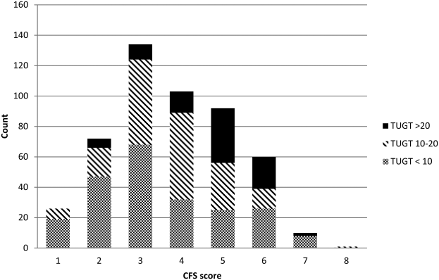
Characteristics According to Frailty Status
Although frail patients were generally similar across definitions (Table 1) in that they were older, had more comorbidities, more hospitalizations in the prior year, and longer index hospitalization lengths of stay than nonfrail patients, patients meeting phenotypic definitions of frailty but not classified as frail on the CFS were younger, had lower Charlson scores, higher EQ‐5D scores, and were discharged with less medications (Table 1).
| Not Frail on Any of the 3 Models, n = 284 | Frail on the CFS Only, n = 80 | Frail on the Fried and/or TUGT but Not the CFS, n = 49 | Frail on CFS and Either Phenotype Model, n = 82 | P Value Comparing the 3 Frailty Columns | |
|---|---|---|---|---|---|
| |||||
| Age, y, mean (95% CI) | 57.3 (55.259.5) | 69.1 (65.872.3) | 63.1 (57.968.3) | 75.8 (72.679.0) | 0.001 |
| Sex, female, no (%) | 118 (41.6) | 49 (61.3) | 27 (55.1) | 56 (68.3) | 0.3 |
| No. of comorbidities, mean (95% CI) | 4.2 (3.84.5) | 6.0 (5.56.6) | 4.0 (3.14.9) | 6.5 (5.87.2) | 0.001 |
| Charlson comorbidity score, mean (95% CI) | 2.4 (2.12.6) | 3.4 (3.03.9) | 2.6 (2.03.2) | 3.8 (3.34.2) | 0.01 |
| No. of patients hospitalized in prior 12 months, no (%) | 93 (32.8) | 44 (55.0) | 27 (55.1) | 54 (65.9) | 0.3 |
| Preadmission living situation, no (%) | 0.01 | ||||
| Living at home independently | 221 (77.8) | 26 (32.5) | 25 (51.0) | 17 (20.7) | |
| Living at home with help | 59 (20.8) | 43 (53.8) | 19 (38.8) | 48 (58.5) | |
| Assisted living or lodge | 4 (1.4) | 11 (13.8) | 5 (10.2) | 17 (20.7) | |
| EQ‐5D overall score, /100, mean (95% CI) | 66.9 (65.068.9) | 62.0 (57.666.4) | 56.6 (51.361.8) | 58.3 (53.962.7) | 0.28 |
| Goals of care in the hospital, no (%) | 0.0001 | ||||
| Resuscitation/ICU | 228 (83.5) | 41 (54.7) | 39 (84.8) | 29 (39.7) | |
| ICU but no resuscitation | 21(7.7) | 17 (22.7) | 1 (2.2) | 16 (21.9) | |
| No ICU, no resuscitation | 23 (8.4) | 17(22.7) | 6 (13.0) | 28 (37.8) | |
| Comfort care | 1 (0.4) | 0 | 0 | 0 | |
| Timed Up and Go Test, s, mean (95% CI) | 10.9 (10.411.3) | 13.9 (12.914.9) | 26.3 (19.033.6) | 30.3 (26.833.7) | 0.0001 |
| Grip strength, kg, mean (95% CI) | 32.1 (30.733.5) | 24.3 (22.3‐ 26.3) | 22.1 (19.924.2) | 17.7 (16.219.1) | 0.0001 |
| Serum albumin, g/L, mean (95% CI) | 34.2 (32.835.5) | 35.0 (33.037.0) | 31.1 (27.934.4) | 33.1 (31.434.9) | 0.07 |
| No. of prescription medications at discharge, mean (95% CI) | 5.2 (4.85.6) | 8.8 (7.99.6) | 6.1 (5.17.1) | 8.2 (7.58.9) | 0.0001 |
| Length of stay, d, median, [IQR] | 5 [37] | 6 [411] | 7 [3.512] | 7 [59] | 0.02 |
Outcomes According to Frailty Status
The overall rate of 30‐day death or hospital readmission was 17.1% (85 patients), primarily as a result of hospital readmissions (81, 16.4%) (Table 2). Although patients classified as frail on the CFS exhibited significantly higher 30‐day readmission/death rates (24.1% vs 13.8% for not frail, P = 0.005) even after adjusting for age and sex (adjusted odds ratio [aOR]: 2.02, 95% CI: 1.19‐3.41) (Table 3), patients meeting either of the phenotypic definitions for frailty but not the CFS definition were not at higher risk for 30‐day readmission/death (aOR: 0.87, 95% CI: 0.34‐2.19) (Table 3). The group at highest risk for 30‐day readmissions/death were those meeting both the CFS and either phenotypic definition of frailty (25.6% vs 13.8% for those not frail, aOR: 2.15, 95% CI: 1.10‐4.19) (Tables 2 and 3). None of the Integrated Discrimination Improvement indices (for modified Fried added to CFS or TUGT added to CFS) were statistically significant, suggesting no net new information was added to predictive models, and there were no appreciable changes in C statistics (Table 3). Neither the modified Fried score nor the TUGT on their own added independent prognostic information to age/sex alone as predictors of postdischarge outcomes. It is noteworthy that the areas under the curve for models using any combination of the frailty definitions plus age and sex were not high (all ranged between 0.55 and 0.60 for the overall cohort and from 0.52 and 0.65 in the elderly). If the frailty definitions were examined as continuous variables rather than dichotomized into frail/not frail, the C statistics were not appreciably better: 0.65 for CFS, 0.58 for TUGT, and 0.60 for modified Fried. Of note, the CFS score with the published cutoff of 5 demonstrated the highest kappa, sensitivity, specificity, and positive predictive value in relation to outcomes.
| Outcomes (Not Mutually Exclusive) | Not Frail on Any of the 3 Models | Frail on the CFS Only | Frail on the Fried and/or TUGT | Frail on CFS and Either Phenotype Model | P Value Comparing the 3 Frailty Columns |
|---|---|---|---|---|---|
| |||||
| Entire cohort | n = 284 | n = 80 | n = 49 | n = 82 | |
| Discharge disposition | 0.002 | ||||
| Live at home independently | 203 (71.5) | 16 (20.0) | 19 (38.8) | 10 (12.2) | |
| Live at home with help | 77 (27.1) | 52 (65.0) | 25 (51.0) | 50 (61.0) | |
| Assisted living or lodge | 4 (9.3) | 12 (15.0) | 5 (10.2) | 22 (26.8) | |
| 30‐day readmission or death | 40 (14.1) | 18 (22.5) | 6 (12.2) | 21 (25.6) | 0.2 |
| 30‐day hospital readmission | 39 (13.8) | 18 (22.5) | 6 (12.2) | 18 (22.0) | 0.31 |
| Death | 5 (1.8) | 3 (3.8) | 1 (2.0) | 4 (4.9) | 0.9 |
| 30‐day ER visit | 66 (23.2) | 30 (37.5) | 12 (24.5) | 23 (17.6) | 0.25 |
| Patients aged 65 years or older | n = 108 | n = 47 | n = 27 | n = 63 | |
| Discharge disposition | 0.03 | ||||
| Live at home independently | 69 (63.9) | 9 (19.2) | 10 (37.0) | 6 (9.5) | |
| Live at home with help | 36 (33.3) | 30 (63.8) | 13 (48.2) | 39(61.9) | |
| Assisted living or lodge | 3 (3.8) | 8 (17.0) | 4 (14.8) | 18 (28.6) | |
| 30‐day readmission or death | 13 (12.0) | 13 (27.7) | 3 (11.1) | 17 (27.0) | 0.22 |
| 30‐day hospital readmission | 12 (11.1) | 13 (27.7) | 3 (11.1) | 14 (22.2) | 0.26 |
| Death | 2 (1.9) | 3 (6.4) | 1 (3.7) | 3 (4.8) | 0.87 |
| 30‐day ER visit | 20 (18.5) | 17 (36.2) | 6 (22.2) | 18 (28.6) | 0.45 |
| Frailty Definition | Adjusted Odds Ratio for 30‐Day Readmission/Death | 95% CI | C Statistic for Model Predicting 30‐Day Readmission/Death Including Age, Sex, and Frailty Definition (95% CI) |
|---|---|---|---|
| |||
| Entire cohort | |||
| CFS (overall) | 2.02 | 1.193.41 | 0.60 (0.530.65) |
| CFS (plus either phenotype model) | 2.15 | 1.104.19 | 0.60 (0.520.64) |
| CFS (but neither phenotype model) | 1.81 | 0.943.48 | 0.60 (0.520.64) |
| Fried | 1.32 | 0.752.30 | 0.55 (0.560.58) |
| TUGT | 1.34 | 0.732.44 | 0.55 (0.460.58) |
| Fried and/or TUGT | 0.87 | 0.342.19 | 0.55 (0.470.58) |
| Patients aged 65 years or older | |||
| CFS (overall) | 3.20 | 1.556.60 | 0.65 (0.560.73) |
| CFS (plus either phenotype model) | 3.20 | 1.337.68 | 0.65 (0.550.72) |
| CFS (but neither phenotype model) | 3.08 | 1.267.47 | 0.65 (0.550.72) |
| Fried | 1.28 | 0.642.56 | 0.52 (0.390.53) |
| TUGT | 1.44 | 0.702.97 | 0.52 (0.390.53) |
| Fried and/or TUGT | 1.41 | 0.722.78 | 0.54 (0.420.56) |
Outcomes According to Frailty Status in the Elderly Subgroup
Although absolute risks of readmission or death were higher in elderly patients than younger patients, the excess risk was largely seen in those elderly patients classified as frail on the CFS. In fact, all of the associations reported above for the entire cohort were in the same direction in the elderly subgroup (Tables 2 and 3).
DISCUSSION
In summary, we found that of patients being discharged from general medical wards who were frail according to at least 1 of the 3 tools we used, only 22% met all 3 frailty case definitions (including only 28% of elderly patients deemed frail by at least 1 definition). There was surprisingly poor correlation between phenotypic markers of frailty such as poor mobility (slow TUGT) or the modified Fried Index and the CFS, even amongt elderly patients. The most clinically useful of the frailty assessment tools (both overall and in those patients who are elderly) appears to be the CFS, because it more accurately identifies those at higher risk of adverse outcomes after discharge, does not require special equipment to conduct, and is faster to do than the phenotypic assessment models we tested. We have also previously demonstrated that the CFS, after a brief training period identical to that used in this study, is reproducible between observers[19] and remains an independent predictor of adverse 30‐day outcomes even after adjusting for age, sex, comorbidities, and the LACE (length of stay, acuity of the admission, comorbidity, emergency room visits during the previous 6 months) score.[14]
Although some[10] have advocated for the use of mobility assessments (such as gait speed) as a frailty marker due to its ease of measurement and objectivity, we found that slow TUGT (which is a marker for mobility and not just slow gait speed) was not an independent prognostic marker for postdischarge outcomes. We hypothesize that the phenotypic models of frailty performed less well than the CFS as they focus on the measurement of particular physical attributes and do not take into account cognitive or psychosocial characteristics or comorbidity burden that also influence postdischarge outcomes. As well, the CFS captures the patients' baseline status prior to acute illness, whereas the phenotypic measures were assessed just prior to discharge and thus may provide less information about eventual recovery potential. Some have suggested that repeating phenotype measures postdischarge might be more informative,[20] but this would reduce clinical applicability a great deal. Certainly, an analysis[21] of the Cardiovascular Health Study cohort demonstrated that cumulative deficit models of frailty (for which the CFS is an accurate proxy[9, 15]) better predicted risk of death than phenotypic models.
Although a number of published studies have shown similar results to ours in that frail patients are at greater risk for death and/or hospitalization,[22, 23, 24] there is surprisingly little literature on the comparative predictive performance of the different frailty instruments and the extent to which they overlap. Cigolle et al.[25] compared 3 frailty scales (the Functional Domain Model, the Burden Model, and the Fried score) in the Health and Retirement Study and, similarly to us, found that although 30.2% were frail on at least 1 of these scales, only 3.1% were deemed frail by all 3. The Conselice Study of Brain Aging[5] also reported that a deficit accumulation model defined a much higher prevalence of frailty (37.6%) than the 11.6% identified using the phenotypic Study of Osteoporotic Fractures (SOF) index based on weight loss, mobility, and level of energy. Another study[26] reported that risk models incorporating either the SOF index or the Fried score exhibited C statistics of only 0.61 for predicting falls in elderly females. A cohort study[27] from 2 English general medical units also found that none of the 5 frailty models was particularly accurate at predicting risk of readmission at 3 months, with C statistics ranging between 0.52 and 0.57. Although frailty assessment at time of hospital admission predicted in‐hospital mortality and length of stay in another English study, it was not independently associated with 30‐day outcomes after adjusting for age, sex, and comorbidities including dementia.[27] To our knowledge, these latter 2 are the only other studies reported to date performed in hospitalized patients to assess whether frailty assessment helps predict postdischarge outcomes. Thus, the poor C statistics we found for all of our frailty tools confirms prior literature that frailty assessment alone is inadequate to accurately identify those patients at highest risk for poor outcomes in the first 30 days after discharge. However, frailty assessment together with consideration of each individual's comorbidities, cognitive status, psychosocial circumstances, and environment can be useful to flag those individuals who may need extra attention postdischarge to optimize outcomes.
Strengths and Limitations
Although this was a prospective cohort study with blinded ascertainment of endpoints (30‐day outcome data were collected by observers who were unaware of the patients' CFS or phenotypic model scores), it is not without limitations. First, the only postdischarge outcomes we assessed were readmission and death, and it would be interesting to evaluate which frailty tools best predict those who are most likely to benefit from home‐care services in the community. Second, as we were interested in 30‐day readmission rates, we excluded long‐term care residents from our study and patients who had foreshortened life expectancy, in essence, the frailest of the frail. Although this reduced the size of any association between frailty and adverse outcomes, we focused this study on the situations where there is clinical equipoise and there is rarely a diagnostic dilemma around the identification of frailty and need for increased services in palliative or long‐term care patients. Third, we did not use exactly the same questionnaires or gait speed assessments as used in the original Fried score description, but as outlined in the Methods section, we used analogous questions on closely related questionnaires to extract the same information. Fourth, some might consider our comparisons biased toward the CFS, as it reflects gestalt clinical impressions (informed by patients and proxies) of frailty status before hospital admission while the Fried score and TUGT were based on patient status just prior to discharge, it may be that the former is a better measure of eventual recovery (and ongoing risk) than the latter measures. If this is the case, for the purposes of targeting interventions to prevent postdischarge complications, it would suggest to us that the CFS is better suited, whereas phenotype tools can be reserved for the postdischarge phase of recovery. By the same token, perhaps serial measures of the CFS and phenotypic tools are more important, as the trajectory of recovery may be most informative for risk prediction.[7] Certainly, if one were interested in changes in functional status during hospitalization,[29] then objective phenotypic measures such as grip strength or TUGT times would seem more appropriate choices. Fifth, some may perceive it as a weakness that we did not restrict our cohort to elderly patients; however, we actually view this as a strength, because frailty is not exclusive to older patients. Sixth, although we restricted this study to patients being discharged from general internal medicine wards, it is worth mentioning that previous studies have shown similar associations between frailty and outcomes in nonmedical hospitalized patients.[19, 22, 23, 24]
In conclusion, we looked at 3 different ways of screening for frailty, 1 being a subjective but well‐validated tool (the CFS) and the other 2 being objective assessments that look at specific phenotypic characteristics. There is a compelling need to find a standardized assessment to determine frailty in both research and clinical settings, and our study provides support for use of the CFS over the Fried or TUGT as screening tools. Standardized frailty assessments should be part of the discharge planning for all medical patients so that extra resources can be properly targeted at those patients at greatest risk for suboptimal transition back to community living.
Acknowledgements
The authors acknowledge Miriam Fradette and Debbie Boyko for their important contributions in data acquisition, as well as all the physicians rotating through the general internal medicine wards for their help in identifying the patients.
Disclosures: Author contributions are as follows: study concept and design: Finlay A. McAlister, Sumit R. Majumdar, and Raj Padwal; acquisition of patients and data: Sara Belga, Darren Lau, Jenelle Pederson, and Sharry Kahlon; analysis of data: Jeff Bakal, Sara Belga, Finlay A. McAlister; first draft of manuscript: Sara Belga and Finlay A. McAlister; critical revision of manuscript: all authors. Funding for this study was provided by an operating grant from Alberta InnovatesHealth Solutions. Alberta InnovatesHealth Solutions had no role in role in the design, methods, subject recruitment, data collections, analysis, or preparation of the article. Finlay A. McAlister and Sumit R. Majumdar hold career salary support from Alberta InnovatesHealth Solutions. Finlay A. McAlister holds the Chair in Cardiovascular Outcomes Research at the Mazankowski Heart Institute, University of Alberta. Sumit R. Majumdar holds the Endowed Chair in Patient Health Management from the Faculty of Medicine and Dentistry, and the Faculty of Pharmacy and Pharmaceutical Sciences, University of Alberta. The authors have no affiliations or financial interests with any organization or entity with a financial interest in the contents of this article. All authors had access to the data and played a role in writing and revising this article. The authors declare no conflicts of interest.
- , , , , . Untangling the concepts of disability, frailty, and comorbidity: implications for improved targeting and care. J Gerontol A Biol Sci Med Sci. 2004;59:255–263.
- , , , , . The identification of frailty: a systematic literature review. J Am Geriatr Soc. 2011;59:2129–2138.
- , , , , . Frailty in elderly people. Lancet. 2013;381:752–762.
- , , , , , . Outcome instruments to measure frailty: a systematic review. Ageing Res Rev. 2011;10:104–114.
- , , , , , . A comparison of frailty indexes for prediction of adverse health outcomes in a elderly cohort. Arch Gerontol Geriatr. 2012;54:16–20.
- , , , et al. Frailty in older adults: evidence for a phenotype. J Gerontol A Biol Sci Med Sci. 2001;56:M146–M156.
- , , , . Prevalence of frailty in community‐dwelling older persons: a systematic review. J Am Geriatr Soc. 2012;60:1487–1492.
- , , . Sex differences in the risk of frailty for mortality independent of disability of chronic diseases. J Am Geriatr Soc. 2005;53:40–47.
- , , . A comparison of two approaches to measuring frailty in elderly people. J Gerontol. 2007;62:738–743.
- , , . A diagnosis of dismobility—giving mobility clinical visibility: a mobility working group recommendation. JAMA. 2014;311:2061–2062.
- , , , et al. Gait speed and survival in older adults. JAMA. 2011;301:50–58.
- , , , et al. Frailty assessment in the cardiovascular care of older adults. J Am Coll Cardiol. 2014;63:747–762.
- , . The timed “Up and Go” test: a test of basic functional mobility for frail elderly persons. J Am Geriatr Soc. 1991;39:142–148.
- , , , et al. Association between frailty and 30‐day outcomes after discharge from hospital. CMAJ. 2015;187:799–804.
- , , , et al. A global clinical measure of fitness and frailty in elderly people. CMAJ. 2005;173:489–495.
- , , , et al. Do muscle mass, muscle density, strength, and physical function similarly influence risk of hospitalization in older adults? J Am Geriatr Soc. 2009;57:1411–1419.
- , . Grip strength in older adults: test‐retest reliability and cutoff for subjective weakness of using the hands in heavy tasks. Arch Phys Med Rehabil. 2010;91:1747–1751.
- , . The PHQ‐9: a new depression measure. Psychiatr Ann. 2002;32:509–515.
- , , , et al. Association between frailty and short‐ and long‐term outcomes among critically ill patients: a multicenter prospective cohort study. CMAJ. 2013;186:e95–e102.
- , . Risk after hospitalization: we have a lot to learn. J Hosp Med. 2015;10:135–136.
- , , , , , . Cumulative deficits better characterize susceptibility to death in elderly people than phenotypic frailty: lessons from the Cardiovascular Health Study. J Am Geriatr Soc. 2008;56:898–903.
- , , . Unplanned hospital readmission and its predictors in patients with chronic conditions. J Formos Med Assoc. 2002;101:779–785.
- , , , et al. Frailty and early hospital readmission after kidney transplant. Am J Transplant. 2013;13:2091–2095.
- , , , , , . Simple frailty score predicts postoperative complications across surgical specialities. Am J Surg. 2013;206:544–550.
- , , , . Comparing models of frailty: the Health and Retirement Study. J Am Geriatr Soc. 2009;57:830–839.
- , , , et al. Comparison of 2 frailty indexes for prediction of falls, disability, fractures, and death in older women. Arch Int Med. 2008;168:382–389.
- , , , , , . The predictive properties of frailty‐rating scales in the acute medical unit. Age Ageing. 2013;42:776–781.
- , , , . Association of the clinical frailty scale with hospital outcomes. QJM. 2015;108:943–949.
- , , . Hospitalization‐associated disability: she was probably able to ambulate, but I'm not sure. JAMA. 2011;306:1782–1793.
Frailty is a state of vulnerability that encompasses a heterogeneous group of people.[1] Because it lacks a precise definition, multiple tools have been developed to identify frailty in both clinical and research settings.[2, 3, 4] Prevalence of frailty depends on the frailty assessment tool used and the population studied, ranging from 4% to 17% when the Fried score[5, 6, 7] is used and from 5% to 44%[5, 7, 8] when cumulative deficit models like the Frailty Index are utilized, with the lower prevalences being in younger community‐dwelling elderly populations and the higher proportions being in older institutionalized populations.
The Frailty Index, also called the Burden or Cumulative Deficit Model, comprises 70 domains that include mobility, mood, function, cognitive impairment, and disease states. It is multidimensional and allows for patients to be categorized on a continuum of frailty, but it is extremely difficult to apply in clinical practice. Recognizing this, Rockwood et al.[9] developed and validated the Clinical Frailty Scale (CFS) in the Canadian Study of Health and Aging. The CFS classifies patients into 1 of 9 categories: very fit, well, managing well, vulnerable, mildly frail (needs help with at least 1 instrumental activity of daily living such as shopping, finances, meal preparation, or housework), moderately frail (needs help with 1 or 2 activities of daily living such as bathing and dressing), severely frail (dependent for personal care), very severely frail (bedbound), and terminally ill. Although this tool is easy to use in clinical practice, it reflects a gestalt impression and requires some clinical judgement.
The Fried score[6] is a prototypical phenotype tool based on 5 criteria that include weight loss, self‐reported exhaustion, low energy expenditure, slowness of gait, and weakness. Recent evidence has suggested that slow gait (or dysmobility) alone may also be a potential screening test for frailty.[10] A recent systematic review[11] demonstrated an association between slow gait (dysmobility) and increased mortality. Dysmobility negatively impacts quality of life and has a strong association with disability resulting in the need for an increased level of care.[12] The Timed Up and Go Test (TUGT) is one method of assessing mobility which is relatively easy to perform, does not require special equipment, and is feasible to use in clinical settings.[13] However, whether impaired mobility predicts outcomes within the first 30 days after hospital discharge (a timeframe highlighted in the Affordable Care Act and used by the Centers for Medicare and Medicaid Services as an important hospital quality indicator) is still uncertain.
The aim of this study was to compare frailty assessments using the CFS and 2 of the most commonly used phenotypic tools (a modified Fried score and the TUGT as a proxy for mobility assessment) to determine which tools best predict postdischarge outcomes.
METHODS
Study Design and Population
As described in detail elsewhere,[14] this was a prospective cohort study that enrolled adult patients (any age older than 18 years) at the time of discharge back to the community from 7 general internal medicine wards in 2 teaching hospitals in Edmonton, Alberta between October 2013 and November 2014. We excluded patients admitted from, or being discharged back to, long‐term care facilities or other acute care hospitals, or from out of the province; patients who were unable to communicate in English; patients with moderate or severe cognitive impairment (scoring 5 or more on the Short Portable Mental Status Questionnaire); or patients with projected life expectancy of less than 3 months. All patients provided written consent, and the study was approved by the Health Research Ethics board of the University of Alberta (project ID Pro00036880).
We assessed the degree of frailty within 24 hours of discharge in 3 ways. First, we used the CFS[9, 15] with patients being asked to rate their best functional status in the week prior to admission. As per the CFS validations studies, scores 5 were defined as frail.[9, 15] Second, we used the TUGT as a proxy for slow gait speed/dysmobility (with >20 seconds defined as abnormal).[13] The TUGT was recorded as the shortest recorded time of the 2 timed trials to get up from a seated position, walk 10 feet and back, and then sit in the chair again. Third, we also determined their Fried score[6] (using the modifications outlined below) and categorized the patients as frail if they scored 3 or more. Of the 5 Fried categories, we assessed weakness by grip strength in their dominant hand using a Jamar handheld dynamometer and weight loss of 10 lb or more in the past year based on patient self‐report; these are identical to the original Fried scale description. Grip strength in the lowest quintile for sex and body mass index was defined as weak grip strength as per convention in the literature, which corresponded to less than 28.5 kg for men and less than 18.5 kg for women.[16, 17] We assessed the other 3 Fried categories in modified fashion as follows. For slow gait, rather than assessing time to walk 15 feet as in the original study and assigning a point to those testing in the lowest quintile for their age/sex, we used the TUGT, because our research personnel were already trained in this test, and we were doing it already as part of the discharge package for all patients.[13] For the Fried category of low activity, we based this on patient self‐report using the relevant questions in the EuroQoL Questionnaire (EQ‐5D); the Fried score used self‐report with a different questionnaire. Finally, for self‐reported exhaustion we used the questions in the Patient Health Questionnaire 9 (PHQ‐9)[18] analogous to those used from the Center for Epidemiological Studies depression scale in the original Fried description. We did this as we were evaluating the PHQ‐9 in our cohort already, and did not want to increase responder burden by presenting them with 2 depression questionnaires.
We followed all patients until 30 days after discharge, and outcome data (all‐cause mortality or all‐cause readmission) were collected by research personnel blinded to the patient's frailty status at discharge using patient/caregiver self‐report and analysis of the provincial electronic health record. We included deaths in or out of the hospital, and all readmissions were unplanned.
We examined the correlation between the CFS score (5 vs 5) and (1) the modified Fried score (3 vs 3) and (2) TUGT (20 seconds vs >20 seconds) using chance corrected kappa coefficients. In our previous article[14] we reported the association between the CFS and readmissions/hospitalizations within 30 days of discharge. In this article we examine whether either the Fried score or TUGT accurately and independently predict postdischarge readmissions/deaths, and whether they add additional prognostic information to the CFS assessment by comparing models with/without each definition using the C statistic and the Integrated Discrimination Improvement index. All analyses were performed using SAS version 9.4 (SAS Institute, Cary, NC), with P values of 0.05 considered statistically significant. Subgroup analysis was done in patients older than 65 years.
RESULTS
Of 1124 potentially eligible patients, 626 were excluded because of patient refusal (n = 227); transfer to/from another hospital, long‐term care facility, or out of province (n = 189); moderate to severe cognitive impairment (n = 88); language barriers (n = 71); or foreshortened life expectancy (n = 51). Another 3 patients withdrew consent prior to outcome assessment. The 495 patients we recruited and had outcome data for had a mean age of 64 years, 19.6% were older than 80 years, 50% were women, and the patients had a mean of 4.2 comorbidities and mean Charlson score of 2.4. The 4 most common reasons for hospital admission were heart failure, pneumonia, chronic obstructive pulmonary disease, and urinary tract infection, and the median length of stay was 5 days (interquartile range: 49 days).
Prevalence of Frailty According to Different Definitions
Although the CFS assessment resulted in 162 (33%) patients being deemed frail, only 82 (51%) of those patients also met the phenotype frailty definition using either the Fried model or the TUGT, and 49 (10%) patients who were not classified as frail on the CFS met either of the phenotypic definitions of frailty (Figure 1). Overall, 211 (43%) patients were frail according to at least 1 assessment, and 46 (9%) met all 3 frailty definitions. In the subgroup of 245 patients older than 65 years, 137 (56%) were frail according to at least 1 assessment, 38 (16%) met all 3 frailty definitions, and 27 (11%) of those patients classified as not frail on the CFS met either phenotypic definition of frailty. Agreement between TUGT and CFS or CFS and Fried was relatively poor with kappas of 0.31 (95% confidence interval [CI]: 0.23‐0.40) and 0.33 (95% CI: 0.25‐0.42), respectively. It is noteworthy that some patients deemed nonfrail on the CFS had slow gait speeds, and most CFS‐frail patients had gait speeds in the nonfrail range (Figure 2).
Characteristics According to Frailty Status
Although frail patients were generally similar across definitions (Table 1) in that they were older, had more comorbidities, more hospitalizations in the prior year, and longer index hospitalization lengths of stay than nonfrail patients, patients meeting phenotypic definitions of frailty but not classified as frail on the CFS were younger, had lower Charlson scores, higher EQ‐5D scores, and were discharged with less medications (Table 1).
| Not Frail on Any of the 3 Models, n = 284 | Frail on the CFS Only, n = 80 | Frail on the Fried and/or TUGT but Not the CFS, n = 49 | Frail on CFS and Either Phenotype Model, n = 82 | P Value Comparing the 3 Frailty Columns | |
|---|---|---|---|---|---|
| |||||
| Age, y, mean (95% CI) | 57.3 (55.259.5) | 69.1 (65.872.3) | 63.1 (57.968.3) | 75.8 (72.679.0) | 0.001 |
| Sex, female, no (%) | 118 (41.6) | 49 (61.3) | 27 (55.1) | 56 (68.3) | 0.3 |
| No. of comorbidities, mean (95% CI) | 4.2 (3.84.5) | 6.0 (5.56.6) | 4.0 (3.14.9) | 6.5 (5.87.2) | 0.001 |
| Charlson comorbidity score, mean (95% CI) | 2.4 (2.12.6) | 3.4 (3.03.9) | 2.6 (2.03.2) | 3.8 (3.34.2) | 0.01 |
| No. of patients hospitalized in prior 12 months, no (%) | 93 (32.8) | 44 (55.0) | 27 (55.1) | 54 (65.9) | 0.3 |
| Preadmission living situation, no (%) | 0.01 | ||||
| Living at home independently | 221 (77.8) | 26 (32.5) | 25 (51.0) | 17 (20.7) | |
| Living at home with help | 59 (20.8) | 43 (53.8) | 19 (38.8) | 48 (58.5) | |
| Assisted living or lodge | 4 (1.4) | 11 (13.8) | 5 (10.2) | 17 (20.7) | |
| EQ‐5D overall score, /100, mean (95% CI) | 66.9 (65.068.9) | 62.0 (57.666.4) | 56.6 (51.361.8) | 58.3 (53.962.7) | 0.28 |
| Goals of care in the hospital, no (%) | 0.0001 | ||||
| Resuscitation/ICU | 228 (83.5) | 41 (54.7) | 39 (84.8) | 29 (39.7) | |
| ICU but no resuscitation | 21(7.7) | 17 (22.7) | 1 (2.2) | 16 (21.9) | |
| No ICU, no resuscitation | 23 (8.4) | 17(22.7) | 6 (13.0) | 28 (37.8) | |
| Comfort care | 1 (0.4) | 0 | 0 | 0 | |
| Timed Up and Go Test, s, mean (95% CI) | 10.9 (10.411.3) | 13.9 (12.914.9) | 26.3 (19.033.6) | 30.3 (26.833.7) | 0.0001 |
| Grip strength, kg, mean (95% CI) | 32.1 (30.733.5) | 24.3 (22.3‐ 26.3) | 22.1 (19.924.2) | 17.7 (16.219.1) | 0.0001 |
| Serum albumin, g/L, mean (95% CI) | 34.2 (32.835.5) | 35.0 (33.037.0) | 31.1 (27.934.4) | 33.1 (31.434.9) | 0.07 |
| No. of prescription medications at discharge, mean (95% CI) | 5.2 (4.85.6) | 8.8 (7.99.6) | 6.1 (5.17.1) | 8.2 (7.58.9) | 0.0001 |
| Length of stay, d, median, [IQR] | 5 [37] | 6 [411] | 7 [3.512] | 7 [59] | 0.02 |
Outcomes According to Frailty Status
The overall rate of 30‐day death or hospital readmission was 17.1% (85 patients), primarily as a result of hospital readmissions (81, 16.4%) (Table 2). Although patients classified as frail on the CFS exhibited significantly higher 30‐day readmission/death rates (24.1% vs 13.8% for not frail, P = 0.005) even after adjusting for age and sex (adjusted odds ratio [aOR]: 2.02, 95% CI: 1.19‐3.41) (Table 3), patients meeting either of the phenotypic definitions for frailty but not the CFS definition were not at higher risk for 30‐day readmission/death (aOR: 0.87, 95% CI: 0.34‐2.19) (Table 3). The group at highest risk for 30‐day readmissions/death were those meeting both the CFS and either phenotypic definition of frailty (25.6% vs 13.8% for those not frail, aOR: 2.15, 95% CI: 1.10‐4.19) (Tables 2 and 3). None of the Integrated Discrimination Improvement indices (for modified Fried added to CFS or TUGT added to CFS) were statistically significant, suggesting no net new information was added to predictive models, and there were no appreciable changes in C statistics (Table 3). Neither the modified Fried score nor the TUGT on their own added independent prognostic information to age/sex alone as predictors of postdischarge outcomes. It is noteworthy that the areas under the curve for models using any combination of the frailty definitions plus age and sex were not high (all ranged between 0.55 and 0.60 for the overall cohort and from 0.52 and 0.65 in the elderly). If the frailty definitions were examined as continuous variables rather than dichotomized into frail/not frail, the C statistics were not appreciably better: 0.65 for CFS, 0.58 for TUGT, and 0.60 for modified Fried. Of note, the CFS score with the published cutoff of 5 demonstrated the highest kappa, sensitivity, specificity, and positive predictive value in relation to outcomes.
| Outcomes (Not Mutually Exclusive) | Not Frail on Any of the 3 Models | Frail on the CFS Only | Frail on the Fried and/or TUGT | Frail on CFS and Either Phenotype Model | P Value Comparing the 3 Frailty Columns |
|---|---|---|---|---|---|
| |||||
| Entire cohort | n = 284 | n = 80 | n = 49 | n = 82 | |
| Discharge disposition | 0.002 | ||||
| Live at home independently | 203 (71.5) | 16 (20.0) | 19 (38.8) | 10 (12.2) | |
| Live at home with help | 77 (27.1) | 52 (65.0) | 25 (51.0) | 50 (61.0) | |
| Assisted living or lodge | 4 (9.3) | 12 (15.0) | 5 (10.2) | 22 (26.8) | |
| 30‐day readmission or death | 40 (14.1) | 18 (22.5) | 6 (12.2) | 21 (25.6) | 0.2 |
| 30‐day hospital readmission | 39 (13.8) | 18 (22.5) | 6 (12.2) | 18 (22.0) | 0.31 |
| Death | 5 (1.8) | 3 (3.8) | 1 (2.0) | 4 (4.9) | 0.9 |
| 30‐day ER visit | 66 (23.2) | 30 (37.5) | 12 (24.5) | 23 (17.6) | 0.25 |
| Patients aged 65 years or older | n = 108 | n = 47 | n = 27 | n = 63 | |
| Discharge disposition | 0.03 | ||||
| Live at home independently | 69 (63.9) | 9 (19.2) | 10 (37.0) | 6 (9.5) | |
| Live at home with help | 36 (33.3) | 30 (63.8) | 13 (48.2) | 39(61.9) | |
| Assisted living or lodge | 3 (3.8) | 8 (17.0) | 4 (14.8) | 18 (28.6) | |
| 30‐day readmission or death | 13 (12.0) | 13 (27.7) | 3 (11.1) | 17 (27.0) | 0.22 |
| 30‐day hospital readmission | 12 (11.1) | 13 (27.7) | 3 (11.1) | 14 (22.2) | 0.26 |
| Death | 2 (1.9) | 3 (6.4) | 1 (3.7) | 3 (4.8) | 0.87 |
| 30‐day ER visit | 20 (18.5) | 17 (36.2) | 6 (22.2) | 18 (28.6) | 0.45 |
| Frailty Definition | Adjusted Odds Ratio for 30‐Day Readmission/Death | 95% CI | C Statistic for Model Predicting 30‐Day Readmission/Death Including Age, Sex, and Frailty Definition (95% CI) |
|---|---|---|---|
| |||
| Entire cohort | |||
| CFS (overall) | 2.02 | 1.193.41 | 0.60 (0.530.65) |
| CFS (plus either phenotype model) | 2.15 | 1.104.19 | 0.60 (0.520.64) |
| CFS (but neither phenotype model) | 1.81 | 0.943.48 | 0.60 (0.520.64) |
| Fried | 1.32 | 0.752.30 | 0.55 (0.560.58) |
| TUGT | 1.34 | 0.732.44 | 0.55 (0.460.58) |
| Fried and/or TUGT | 0.87 | 0.342.19 | 0.55 (0.470.58) |
| Patients aged 65 years or older | |||
| CFS (overall) | 3.20 | 1.556.60 | 0.65 (0.560.73) |
| CFS (plus either phenotype model) | 3.20 | 1.337.68 | 0.65 (0.550.72) |
| CFS (but neither phenotype model) | 3.08 | 1.267.47 | 0.65 (0.550.72) |
| Fried | 1.28 | 0.642.56 | 0.52 (0.390.53) |
| TUGT | 1.44 | 0.702.97 | 0.52 (0.390.53) |
| Fried and/or TUGT | 1.41 | 0.722.78 | 0.54 (0.420.56) |
Outcomes According to Frailty Status in the Elderly Subgroup
Although absolute risks of readmission or death were higher in elderly patients than younger patients, the excess risk was largely seen in those elderly patients classified as frail on the CFS. In fact, all of the associations reported above for the entire cohort were in the same direction in the elderly subgroup (Tables 2 and 3).
DISCUSSION
In summary, we found that of patients being discharged from general medical wards who were frail according to at least 1 of the 3 tools we used, only 22% met all 3 frailty case definitions (including only 28% of elderly patients deemed frail by at least 1 definition). There was surprisingly poor correlation between phenotypic markers of frailty such as poor mobility (slow TUGT) or the modified Fried Index and the CFS, even amongt elderly patients. The most clinically useful of the frailty assessment tools (both overall and in those patients who are elderly) appears to be the CFS, because it more accurately identifies those at higher risk of adverse outcomes after discharge, does not require special equipment to conduct, and is faster to do than the phenotypic assessment models we tested. We have also previously demonstrated that the CFS, after a brief training period identical to that used in this study, is reproducible between observers[19] and remains an independent predictor of adverse 30‐day outcomes even after adjusting for age, sex, comorbidities, and the LACE (length of stay, acuity of the admission, comorbidity, emergency room visits during the previous 6 months) score.[14]
Although some[10] have advocated for the use of mobility assessments (such as gait speed) as a frailty marker due to its ease of measurement and objectivity, we found that slow TUGT (which is a marker for mobility and not just slow gait speed) was not an independent prognostic marker for postdischarge outcomes. We hypothesize that the phenotypic models of frailty performed less well than the CFS as they focus on the measurement of particular physical attributes and do not take into account cognitive or psychosocial characteristics or comorbidity burden that also influence postdischarge outcomes. As well, the CFS captures the patients' baseline status prior to acute illness, whereas the phenotypic measures were assessed just prior to discharge and thus may provide less information about eventual recovery potential. Some have suggested that repeating phenotype measures postdischarge might be more informative,[20] but this would reduce clinical applicability a great deal. Certainly, an analysis[21] of the Cardiovascular Health Study cohort demonstrated that cumulative deficit models of frailty (for which the CFS is an accurate proxy[9, 15]) better predicted risk of death than phenotypic models.
Although a number of published studies have shown similar results to ours in that frail patients are at greater risk for death and/or hospitalization,[22, 23, 24] there is surprisingly little literature on the comparative predictive performance of the different frailty instruments and the extent to which they overlap. Cigolle et al.[25] compared 3 frailty scales (the Functional Domain Model, the Burden Model, and the Fried score) in the Health and Retirement Study and, similarly to us, found that although 30.2% were frail on at least 1 of these scales, only 3.1% were deemed frail by all 3. The Conselice Study of Brain Aging[5] also reported that a deficit accumulation model defined a much higher prevalence of frailty (37.6%) than the 11.6% identified using the phenotypic Study of Osteoporotic Fractures (SOF) index based on weight loss, mobility, and level of energy. Another study[26] reported that risk models incorporating either the SOF index or the Fried score exhibited C statistics of only 0.61 for predicting falls in elderly females. A cohort study[27] from 2 English general medical units also found that none of the 5 frailty models was particularly accurate at predicting risk of readmission at 3 months, with C statistics ranging between 0.52 and 0.57. Although frailty assessment at time of hospital admission predicted in‐hospital mortality and length of stay in another English study, it was not independently associated with 30‐day outcomes after adjusting for age, sex, and comorbidities including dementia.[27] To our knowledge, these latter 2 are the only other studies reported to date performed in hospitalized patients to assess whether frailty assessment helps predict postdischarge outcomes. Thus, the poor C statistics we found for all of our frailty tools confirms prior literature that frailty assessment alone is inadequate to accurately identify those patients at highest risk for poor outcomes in the first 30 days after discharge. However, frailty assessment together with consideration of each individual's comorbidities, cognitive status, psychosocial circumstances, and environment can be useful to flag those individuals who may need extra attention postdischarge to optimize outcomes.
Strengths and Limitations
Although this was a prospective cohort study with blinded ascertainment of endpoints (30‐day outcome data were collected by observers who were unaware of the patients' CFS or phenotypic model scores), it is not without limitations. First, the only postdischarge outcomes we assessed were readmission and death, and it would be interesting to evaluate which frailty tools best predict those who are most likely to benefit from home‐care services in the community. Second, as we were interested in 30‐day readmission rates, we excluded long‐term care residents from our study and patients who had foreshortened life expectancy, in essence, the frailest of the frail. Although this reduced the size of any association between frailty and adverse outcomes, we focused this study on the situations where there is clinical equipoise and there is rarely a diagnostic dilemma around the identification of frailty and need for increased services in palliative or long‐term care patients. Third, we did not use exactly the same questionnaires or gait speed assessments as used in the original Fried score description, but as outlined in the Methods section, we used analogous questions on closely related questionnaires to extract the same information. Fourth, some might consider our comparisons biased toward the CFS, as it reflects gestalt clinical impressions (informed by patients and proxies) of frailty status before hospital admission while the Fried score and TUGT were based on patient status just prior to discharge, it may be that the former is a better measure of eventual recovery (and ongoing risk) than the latter measures. If this is the case, for the purposes of targeting interventions to prevent postdischarge complications, it would suggest to us that the CFS is better suited, whereas phenotype tools can be reserved for the postdischarge phase of recovery. By the same token, perhaps serial measures of the CFS and phenotypic tools are more important, as the trajectory of recovery may be most informative for risk prediction.[7] Certainly, if one were interested in changes in functional status during hospitalization,[29] then objective phenotypic measures such as grip strength or TUGT times would seem more appropriate choices. Fifth, some may perceive it as a weakness that we did not restrict our cohort to elderly patients; however, we actually view this as a strength, because frailty is not exclusive to older patients. Sixth, although we restricted this study to patients being discharged from general internal medicine wards, it is worth mentioning that previous studies have shown similar associations between frailty and outcomes in nonmedical hospitalized patients.[19, 22, 23, 24]
In conclusion, we looked at 3 different ways of screening for frailty, 1 being a subjective but well‐validated tool (the CFS) and the other 2 being objective assessments that look at specific phenotypic characteristics. There is a compelling need to find a standardized assessment to determine frailty in both research and clinical settings, and our study provides support for use of the CFS over the Fried or TUGT as screening tools. Standardized frailty assessments should be part of the discharge planning for all medical patients so that extra resources can be properly targeted at those patients at greatest risk for suboptimal transition back to community living.
Acknowledgements
The authors acknowledge Miriam Fradette and Debbie Boyko for their important contributions in data acquisition, as well as all the physicians rotating through the general internal medicine wards for their help in identifying the patients.
Disclosures: Author contributions are as follows: study concept and design: Finlay A. McAlister, Sumit R. Majumdar, and Raj Padwal; acquisition of patients and data: Sara Belga, Darren Lau, Jenelle Pederson, and Sharry Kahlon; analysis of data: Jeff Bakal, Sara Belga, Finlay A. McAlister; first draft of manuscript: Sara Belga and Finlay A. McAlister; critical revision of manuscript: all authors. Funding for this study was provided by an operating grant from Alberta InnovatesHealth Solutions. Alberta InnovatesHealth Solutions had no role in role in the design, methods, subject recruitment, data collections, analysis, or preparation of the article. Finlay A. McAlister and Sumit R. Majumdar hold career salary support from Alberta InnovatesHealth Solutions. Finlay A. McAlister holds the Chair in Cardiovascular Outcomes Research at the Mazankowski Heart Institute, University of Alberta. Sumit R. Majumdar holds the Endowed Chair in Patient Health Management from the Faculty of Medicine and Dentistry, and the Faculty of Pharmacy and Pharmaceutical Sciences, University of Alberta. The authors have no affiliations or financial interests with any organization or entity with a financial interest in the contents of this article. All authors had access to the data and played a role in writing and revising this article. The authors declare no conflicts of interest.
- , , , , . Untangling the concepts of disability, frailty, and comorbidity: implications for improved targeting and care. J Gerontol A Biol Sci Med Sci. 2004;59:255–263.
- , , , , . The identification of frailty: a systematic literature review. J Am Geriatr Soc. 2011;59:2129–2138.
- , , , , . Frailty in elderly people. Lancet. 2013;381:752–762.
- , , , , , . Outcome instruments to measure frailty: a systematic review. Ageing Res Rev. 2011;10:104–114.
- , , , , , . A comparison of frailty indexes for prediction of adverse health outcomes in a elderly cohort. Arch Gerontol Geriatr. 2012;54:16–20.
- , , , et al. Frailty in older adults: evidence for a phenotype. J Gerontol A Biol Sci Med Sci. 2001;56:M146–M156.
- , , , . Prevalence of frailty in community‐dwelling older persons: a systematic review. J Am Geriatr Soc. 2012;60:1487–1492.
- , , . Sex differences in the risk of frailty for mortality independent of disability of chronic diseases. J Am Geriatr Soc. 2005;53:40–47.
- , , . A comparison of two approaches to measuring frailty in elderly people. J Gerontol. 2007;62:738–743.
- , , . A diagnosis of dismobility—giving mobility clinical visibility: a mobility working group recommendation. JAMA. 2014;311:2061–2062.
- , , , et al. Gait speed and survival in older adults. JAMA. 2011;301:50–58.
- , , , et al. Frailty assessment in the cardiovascular care of older adults. J Am Coll Cardiol. 2014;63:747–762.
- , . The timed “Up and Go” test: a test of basic functional mobility for frail elderly persons. J Am Geriatr Soc. 1991;39:142–148.
- , , , et al. Association between frailty and 30‐day outcomes after discharge from hospital. CMAJ. 2015;187:799–804.
- , , , et al. A global clinical measure of fitness and frailty in elderly people. CMAJ. 2005;173:489–495.
- , , , et al. Do muscle mass, muscle density, strength, and physical function similarly influence risk of hospitalization in older adults? J Am Geriatr Soc. 2009;57:1411–1419.
- , . Grip strength in older adults: test‐retest reliability and cutoff for subjective weakness of using the hands in heavy tasks. Arch Phys Med Rehabil. 2010;91:1747–1751.
- , . The PHQ‐9: a new depression measure. Psychiatr Ann. 2002;32:509–515.
- , , , et al. Association between frailty and short‐ and long‐term outcomes among critically ill patients: a multicenter prospective cohort study. CMAJ. 2013;186:e95–e102.
- , . Risk after hospitalization: we have a lot to learn. J Hosp Med. 2015;10:135–136.
- , , , , , . Cumulative deficits better characterize susceptibility to death in elderly people than phenotypic frailty: lessons from the Cardiovascular Health Study. J Am Geriatr Soc. 2008;56:898–903.
- , , . Unplanned hospital readmission and its predictors in patients with chronic conditions. J Formos Med Assoc. 2002;101:779–785.
- , , , et al. Frailty and early hospital readmission after kidney transplant. Am J Transplant. 2013;13:2091–2095.
- , , , , , . Simple frailty score predicts postoperative complications across surgical specialities. Am J Surg. 2013;206:544–550.
- , , , . Comparing models of frailty: the Health and Retirement Study. J Am Geriatr Soc. 2009;57:830–839.
- , , , et al. Comparison of 2 frailty indexes for prediction of falls, disability, fractures, and death in older women. Arch Int Med. 2008;168:382–389.
- , , , , , . The predictive properties of frailty‐rating scales in the acute medical unit. Age Ageing. 2013;42:776–781.
- , , , . Association of the clinical frailty scale with hospital outcomes. QJM. 2015;108:943–949.
- , , . Hospitalization‐associated disability: she was probably able to ambulate, but I'm not sure. JAMA. 2011;306:1782–1793.
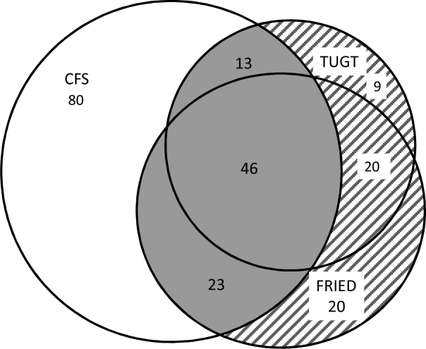
Hospital‐Wide Readmission Rates
The hospital‐wide all‐cause 30‐day readmission rate is a key quality measure associated with patient outcomes, cost of care, and wasted hospital resources.[1] The estimated 20% readmission rate of Medicare patients and the associated $17 billion annual cost of readmissions led the Centers for Medicare and Medicaid Services (CMS) to implement policies that limit reimbursement for 30‐day unplanned readmissions and thus place hospitals with high readmission rates at financial risk.[1, 2]
The variation in readmission rates between hospitals is well documented in the literature.[3, 4] Singh et al. found that 9.3% of the variation in readmissions can be explained by hospital characteristics.[4] Hospital factors associated with lower readmission rates include not‐for‐profit ownership, hospital size, and nursing staffing levels.[5, 6, 7] Other studies found an association between environmental factors such as the percent of patients living under the poverty line and higher readmission rates.[7] The recent publicly available CMS data on readmission rates allows us to further our understanding of hospital characteristics that explain the variation in readmission rates. In this article, we are specifically interested in hospitalist staffing levels and hospital‐physician arrangements such as physician integration level and physician ownership. Moreover, we are interested in novel organizational variables, specifically, the adoption of a medical home model, which has been ignored by previous research. Medical homes are associated with better quality[8]; hospitals that already adopted the medical home model might be better equipped to coordinate care after the patients are discharged.
In recent years, the number of hospitals relying on hospitalists to provide inpatient care has been on the rise. As more hospitals employ hospitalists, it is important to understand how hospitalist staffing levels are associated with quality. Previous studies have linked hospitalists with lower hospital mortality rates,[7] lower cost of care,[9, 10] and lower readmission rates.[10, 11] Goodrich et al., on the other hand, did not find a significant relationship between the presence of hospitalists and mortality or readmission rates.[12] In a recent study, hospitalists indicated that heavy workloads limited the time they had available to communicate with patients, which negatively influenced quality and patient satisfaction, and resulted in delayed admissions and discharges.[13]
The main objective of this article was therefore to study the association between hospitalist staffing levels and hospital‐wide all‐cause readmission rates. Most empirical studies examining the relationship between hospitalist staffing and quality of inpatient care have predominantly focused on whether the presence of hospitalists who provided care at a hospital influenced mortality or readmissions.[11, 12] In this article, we contribute to the literature by examining how staffing levels measured by the ratio of hospitalists to general medical and surgical beds is associated with 30‐day readmission rates. We predict that there is a positive association between readmission rates and hospitalists per bed.
Hospitals have a broad range of contractual arrangements or integration levels with physicians, with employment being the highest level. A hospital can rely on physicians who have admitting privileges but are not salaried employees of the hospital to treat a large portion of its inpatient population. In the past few years, with the passage of the Patient Protection and Affordable Care Act (2010) and the shift in reimbursement towards Value Based Purchasing (VBP), more hospitals are choosing to ensure that physicians are strongly integrated within the hospital by adopting an employment‐based model. Moreover, hospitals view physician employment as a strategic move that will help ensure or expand their market share.[14] For instance, the number of surgeons who identified as self‐employed dropped from 48% in 2001 to 28% in 2011, and this reduction is attributed to the shift toward hospital employment of physicians.[15] Despite the evolving models of hospital‐physician arrangements, little is understood on how the adoption of the integrated salary model, in addition to the equity and foundation models, which are classified by Baker et al. as the highest level of integration, influence quality.[16] Therefore, another objective of this article was to examine the association between hospital‐physician arrangements and all‐cause unplanned readmission rates.
METHODS
Data Source and Sample
Data from the American Hospital Association (AHA) Annual Survey (2013), CMS Hospital Compare (October 2013), and Area Health Resource File (2013) were merged to analyze the association between readmission rates with hospital characteristics and environmental factors. We limited the analysis to private (nonpublic) hospitals with no missing data. Our final sample consisted of 1756 hospitals. Of the hospitals in our sample, 14% were for profit, 70% were nonteaching, 23% were minor teaching, 7% were major teaching hospitals, 73% belonged to a system, and 31% were classified as small hospitals. Table 1 provides descriptive statistics for all the variables included in the analysis.
| Variable | Value | Data Source |
|---|---|---|
| ||
| 30‐day all‐cause readmissions, median (IQR) | 15.8% (15.2%16.5%) | Centers for Medicare and Medicaid Services |
| Hospitalists per general medicine and surgical beds, median (IQR) | 0.09 (0.060.15) | American Hospital Association |
| RNs per 100 inpatient days, median (IQR) | 0.84 (0.6610.10) | American Hospital Association |
| Medicare admissions, median (IQR) | 48.45% (40.84%55.14%) | American Hospital Association |
| Medicaid admissions, median (IQR) | 16.45% (11.06%22.76%) | American Hospital Association |
| Competition, median (IQR) | 0.56 (0.230.83) | American Hospital Association |
| Unemployment, median (IQR) | 2.9% (2.54%3.37%) | Area Resource File |
| Fully integrated | American Hospital Association | |
| Yes | 51% | |
| No | 49% | |
| Physician ownership | American Hospital Association | |
| Physician partial or complete ownership | 5% | |
| No physician ownership | 95% | |
| Established medical home program | American Hospital Association | |
| Yes | 29% | |
| No | 71% | |
| High technology | American Hospital Association | |
| Yes | 40% | |
| No | 60% | |
| Teaching level | American Hospital Association | |
| Nonteaching | 70% | |
| Minor teaching | 23% | |
| Major teaching | 7% | |
| Size | American Hospital Association | |
| Small | 31% | |
| Medium | 34% | |
| Large | 35% | |
| Ownership | American Hospital Association | |
| For profit | 14% | |
| Not for profit | 86% | |
| Critical access hospital | American Hospital Association | |
| Yes | 11% | |
| No | 89% | |
| System membership | American Hospital Association | |
| Yes | 73% | |
| No | 27% | |
Variables
Dependent Variable
Risk standardized 30‐day hospital‐wide all‐cause readmission rates (HWR) were obtained from CMS. This measure was publicly reported in October 2013. The HWR is estimated using standardized risk ratios at the hospital level for the following 5 discharge diagnosis groups: surgery/gynecology, neurology, cardiorespiratory, cardiovascular, and general medicine.[17] The measure adjusts, in addition to a hospital's case mix, for patients' ages, principal discharge diagnoses, and comorbidities.[17] HWR is calculated as a predicted‐to‐expected readmissions ratio. Predicted and expected readmissions were calculated for each of the 5 groups for each hospital using each hospital's patient mix and a hospital random effects estimate. A standardized readmission ratio was then derived by dividing predicted readmissions by expected readmissions for each group for each hospital. A single hospital score was obtained by multiplying the volume‐weighted logarithmic average of the 5 diagnostic groups by the average national readmission rate.[18]
Independent Variables
The primary independent variable of interest to this study is hospitalist staffing levels. We calculate the staffing levels of hospitalists by dividing the full‐time equivalent (FTE) of hospitalists by the number of general medical and surgical beds. FTE hospitalists are calculated by the AHA Annual Survey database (2013) as the sum of full‐time hospitalists and 0.5*number of part‐time hospitalists. In addition to hospitalist staffing levels, a main predictors is whether the hospital fully integrates physicians or not. We follow Baker et al. in our classification of full integration. Baker et al. define fully integrated hospitals as those that adopted 1 of the following models with their physicians: integrated salary, foundation or equity model.[16] We predict that fully integrated hospitals are more likely to have better readmission rates. Another key physician variable that is likely to influence outcomes is physician partial or full ownership of the hospital. Ownership aligns physicians' incentives with hospital performance[19] and is therefore likely to be associated with better readmission rates. We also include a dichotomous variable that indicates whether a hospital has an established medical home program or not. Medical homes indicate an organizational culture that is patient centered and committed to continuity and coordination of care; all of which are important for better quality. We predict that the presence of a medical home model will be associated with better readmission rates.
Control Variables
We control for registered nurses per 100 inpatient days ratio, critical access designation, Medicare share of hospital admissions, Medicaid share of hospital admissions, teaching status, size, and technology level. Previous research indicates that these variables are associated with patient outcomes.[20, 21] We follow the Aiken et al. characterization of teaching status: hospitals with no residency programs (nonteaching), hospitals with a resident‐to‐bed ratio of 1 to 4 or less (minor teaching), and hospitals with a resident‐to‐bed ratio of more than 1 to 4 (major teaching).[20] We also classify hospitals as small if they have less than 100 beds, medium if they have 101 to 250 beds, and large if they have more than 250 beds. We modify the Aiken et al. classification of technology level and control for the level of technology adopted at a hospital by classifying hospitals as high technology if they offer any of the following services: any major organ transplant, computer‐assisted orthopedic surgery, or electron beam computed tomography.[21] We also control for 2 market level variables: (1) competition estimated by the county level Herfindahl‐Hirschman Index (HHI) and (2) the percentage of individuals in the county who are unemployed. Unemployment rates are derived from the Area Health Resource File (2013). HHI is calculated by summing the squares of market shares of admissions. For ease of interpretation, competition is coded as 1‐HHI.
Statistical Analysis
We ran a multivariate ordinary least squares (OLS) regression on Stata 12 (StataCorp, College Station, TX) to assess the relationship between 30‐day all‐cause readmissions and hospitalist staffing levels, physician integration, physician ownership, and other organizational characteristics. We checked for multicollinearity by using a variance inflation factor (VIF). The VIF of all independent variables was less than 10, and therefore multicollinearity was not of concern to this analysis.
RESULTS
Among our sample of 1756 hospitals, the median 30‐day all‐cause readmission rate was 16%, with the middle 50% of hospitals with readmission rates between 15.2% and 16.5%. All of the hospitals in this study reported that hospitalists provide care at the hospitals. The median Medicare share of hospital admissions was 48.46%, and the median Medicaid share of hospital admissions was 16.4%. Fifty‐one percent of the hospitals in our sample were fully integrated. Fifty percent of hospitals had 9 or fewer hospitalists per 100 general medical and surgical beds. Only 5% of the hospitals had partial or full physician ownership. Twenty‐nine percent of hospitals had an established medical home program. Table 1 provides summary statistics and the data sources of all the variables included in the study.
To compare readmission rates, we created a dummy variable that divided the sample into 2 categories: hospitals with low hospitalist staffing levels (hospitalists per general medical and surgical beds is less than the median) and high hospitalist staffing (hospitalists per general medical and surgical bed ratio is more than the median). We then used t tests to compare all‐cause readmission rates between hospitals with low and high hospitalist staffing levels, physician owned versus nonphysician owned, and fully integrated versus not fully integrated. We also used single‐factor analysis of variance (ANOVA) to compare readmission rates between nonteaching, minor teaching, and major teaching hospitals. Results are displayed in Table 2. There was a significant difference in the mean readmission rates between hospitals with low hospitalist staffing levels (mean readmission rate = 16.06%) versus high staffing levels (mean readmission rate = 15.72%). The mean readmission rate for physician‐owned hospitals was significantly lower than for nonphysician‐owned hospitals (15.46% vs 15.9%). Also, fully integrated hospitals had a lower readmission rate than hospitals where physicians were not fully integrated (15.93% vs 15.86%). Based on the ANOVA results, there was a significant difference between teaching levels. According to a Tukey honest significant difference post hoc test, there was no significant difference between nonteaching and minor teaching hospitals, but the readmission rate was significantly higher in major teaching hospitals (nonteaching = 15.83%, minor teaching = 15.76%, major teaching = 16.9%).
| Variable | Readmission Rates | P Value |
|---|---|---|
| Hospitalist staffing levels | ||
| Low | 16.06% | 0.00 |
| High | 15.72% | |
| Physician ownership | ||
| Fully or partially physician‐owned hospitals | 15.46% | 0.00 |
| Nonphysician‐owned hospitals | 15.9 % | |
| Physician integration | ||
| Fully integrated hospitals | 15.86% | 0.00 |
| Nonintegrated hospitals | 15.93% | |
| Teaching status | ||
| Nonteaching hospitals | 15.83% | 0.00 |
| Minor teaching hospitals | 15.76% | |
| Major teaching hospitals | 16.9% |
The OLS regression model was significant and explained 16% of the variability in readmission rates (Table 3). Higher hospitalists staffing levels were associated with lower 30‐day all cause readmission rates (P = 0.00). The addition of 1 hospitalist per general and surgical bed was associated with a 0.77 percentage points decrease in adjusted readmission rates. In terms of hospital‐physician arrangements, fully integrated hospitals had adjusted 30‐day all‐cause readmission rates 0.09 percentage points lower than nonfully integrated hospitals (P = 0.08). Physician partial or full ownership was significantly associated with lower readmission rates (P = 0.00); hospitals partially or fully owned by physicians had adjusted readmission rates 0.36 percentage points lower than nonphysician‐owned hospitals.
| Variable | Coefficient | Standard Error | P Value |
|---|---|---|---|
| |||
| Hospitalists per general and surgical beds | 0.77 | 0.172 | 0.00 |
| Full integration | 0.086 | 0.049 | 0.08 |
| Physician ownership | 0.355 | 0.119 | 0.00 |
| RNs per 100 inpatient days | 0.174 | 0.050 | 0.00 |
| Established medical home program | 0.132 | 0.057 | 0.02 |
| Medicare admissions | 0.063 | 0.002 | 0.21 |
| Medicaid admissions | 0.015 | 0.003 | 0.00 |
| Competition | 0.115 | 0.08 | 0.17 |
| Unemployment | 0.244 | 0.037 | 0.00 |
| System membership | 0.041 | 0.055 | 0.45 |
| Teaching level | |||
| Minor teaching | 0.007 | 0.066 | 0.92 |
| Major teaching | 1.032 | 0.106 | 0.00 |
| Size | |||
| Medium | 0.032 | 0.071 | 0.66 |
| Large | 0.066 | 0.085 | 0.44 |
| For‐profit ownership | 0.206 | 0.078 | 0.01 |
| High technology | 0.077 | 0.055 | 0.17 |
| Critical access hospital | 0.202 | 0.092 | 0.03 |
Based on the regression analysis, major teaching hospitals on average had adjusted readmission rates 1.03 percentage point higher than nonteaching hospitals (P = 0.000), whereas there was no significant difference between minor and nonteaching hospitals (P > 0.1). As the number of registered nurses (RNs) per 100 inpatient days increased by 1, readmission rates dropped by 0.17 (P = 0.00). Hospitals with higher Medicaid shares of admission had significantly higher readmission rates (P 0.05). Hospitals located in counties with higher unemployment rates also had higher readmission rates (P = 0.000), whereas market competition had no significant association with readmissions. For‐profit hospitals had adjusted readmission rates 0.21 percentage points higher than not‐for‐profit hospitals (P = 0.01). Finally, hospitals that have adopted a medical home model had significantly lower readmission rates (P = 0.02); hospitals with an established medical home model had adjusted readmission rates 0.17 percentage points lower than their counterparts.
DISCUSSION
In the era of VBP and mounting pressures on hospitals to improve quality and lower cost, it is important to understand the association between modifiable hospital characteristics, such as hospitalist staffing levels, and unmodifiable characteristics, such as teaching status and size, with quality of care. There are many factors that can contribute to higher readmission rates. Some of these factors are hospital related and others are patient related, such as the environment in which a patient resides. Benbassat and Taragin argue that 9% to 48% of hospital readmissions are avoidable and are related to factors such as inadequate resolution of the problem the patient was admitted for and poor discharge care.[22] In this article, we have focused on hospital and market factors. Our main variables of interest were hospitalist staffing level, physician full integration, physician ownership, and the adoption of the medical home model at the hospital. Moreover, we examined the association between the hospital environment, specifically, market competition, and the patient environment, specifically, unemployment rates, with readmission rates.
Hospitalists' provision of inpatient care has been on the rise. From 1997 to 2006, the likelihood of receiving inpatient care from a hospitalist grew by 29.2% per year.[23] Based on AHA (2013) data, 65% of hospitals reported that hospitalists provided care at the hospital. The main driver behind the adoption of the hospitalists' model is the positive role hospitalists play in improving hospital efficiency and their familiarity and specialization in hospital care.[24] However, concerns exist that hospitalists might negatively influence patient outcomes given the discontinuity of care that occurs once the patient is discharged from the hospital and back to the care of their primary care physician.[25] Based on our analysis though, higher hospitalist staffing levels were associated with lower readmission rates. Therefore, to better understand the relationship between hospitalists and quality, it is important to account for staffing levels, not merely whether hospitalists provide care at the hospital or not. Higher patient load per hospitalist might still improve hospital efficiency by lowering costs, but is it likely to impede the quality of care provided by hospitalists. This is not surprising given similar findings, including in this article, which document a similar positive relationship between nursing staffing levels and quality.
Hospitals utilize various arrangements with physicians that range from employment to more relaxed arrangements such as physicians with privileges who are neither employed by the hospital nor under individual or group contracts. Historically, the main incentive for hospitals to integrate physicians was referrals to hospital services and specialties.[16, 26] The Affordable Care Act, however, provided further incentives, such as ease of care coordination, physicians' involvement, and commitment to quality improvement and cost‐containment efforts. Based on this study, hospitals that were classified as fully integrated had lower readmission rates. Also, hospitals partially or fully owned by physicians had better readmission rates. These findings indicate that hospital‐physician arrangements play a significant role not only in influencing efficiency and market share but also patient outcomes. Physician integration and physician ownership align physicians' financial incentives with those of the hospital. For instance, given the recent changes in reimbursement and the shift toward VBP, physician income in physician‐owned hospitals is at risk if the hospital has poor patient outcomes.
Other significant predictors of readmission rates included the adoption of the medical home model and RN staffing levels. Hospitals that adopted a medical home model and had a higher registered nurse‐to‐inpatient days ratio had significantly better readmission rates. The finding on the adoption of the medical home model is especially important. Previous research indicates that patient‐centered medical homes are associated with lower emergency room visits but not necessarily lower admissions.[27] Our findings indicate that medical homes might play a role in lowering readmission rates, and therefore this outcome needs to be included in studies examining the performance of medical homes. Critical access hospitals and those with higher admissions share of Medicaid patients had worst readmission rates. Finally, hospitals located in counties with higher unemployment rates also had the worst readmission rates. This finding is not surprising and is consistent with previous research, which indicates that the patients' environment and social risk factors play a significant role.
This article contributes to our understanding of readmission rates despite its several limitations, which include the measurement of hospitalist staffing levels based on general medical and surgical beds rather than general medicine admissions. Moreover, some hospitals had missing data on key variables, which warranted their exclusion from this study. In conclusion, many structural, operational and market‐level factors influence all‐cause readmission rates. However, some of these variables are modifiable and can thus be adjusted by a hospital to improve readmission rates. These variables include hospitalists and registered nurse staffing levels; physician integration through the salaried, equity, or foundation model; and the adoption of a medical home model.
Disclosure
Nothing to report.
- , , . Medicare's readmissions‐reduction program—a positive alternative. N Engl J Med. 2012;366:1364–1366.
- , , , et al. Impact of hospital population case‐mix, including poverty, on hospital all‐cause and infection‐related 30‐day readmission rates. Clin Infect Dis. 2015;31(2):1235–1243.
- , , , et al. Patterns of hospital performance in acute myocardial infarction and heart failure 30‐day mortality and readmission. Circ Cardiovasc Qual Outcomes. 2009;2:407–413.
- , , , , . Variation in the risk of readmission among hospitals: the relative contribution of patient, hospital and inpatient provider characteristics. J Gen Intern Med. 2014;29:572–578.
- , . A path forward on Medicare readmissions. N Engl J Med. 2013;368:1175–1177.
- , , . Hospitals with higher nurse staffing had lower odds of readmissions penalties than hospitals with lower staffing. Health Aff (Millwood). 2013;32:1740–1747.
- , , , , . Variation in surgical‐readmission rates and quality of hospital care. N Engl J Med. 2013;369:1134–1142.
- , , , et al. Value and the medical home: effects of transformed primary care. Am J Manag Care. 2010;16.8:607–614.
- , , , , , . Effects of hospitalists on cost, outcomes, and patient satisfaction in a rural health system. Am J Med. 2000;108:621–626.
- , , , , . Effect of hospitalist workload on the quality and efficiency of care. JAMA Intern Med. 2014;174:786–793.
- , , . Association of hospitalist presence and hospital‐level outcome measures among Medicare patients. J Hosp Med. 2014;9:1–6.
- , , , , . Hospitalist utilization and hospital performance on 6 publicly reported patient outcomes. J Hosp Med. 2012;7:482–488.
- , , , . Impact of attending physician workload on patient care: a survey of hospitalists. JAMA Intern Med. 2013;173:375–377.
- , , . Rising hospital employment of physicians: better quality, higher costs. Issue Brief Cent Stud Health Syst Change. 2011;136:1–4.
- , , , et al. The employed surgeon: a changing professional paradigm. JAMA Surg. 2013;148:323–328.
- , , . Vertical integration: hospital ownership of physician practices is associated with higher prices and spending. Health Aff (Millwood). 2014;33:756–763.
- , , , et al. Hospital‐wide (all‐condition) 30‐day risk‐standardized readmission measure: Yale New Haven Health Services Corporation. Center for Outcomes Research 161(10 suppl):S66–S75.
- , . Hospital‐physician collaboration: landscape of economic integration and impact on clinical integration. Milbank Q. 2008;86(3):375–434.
- , , , , . Effects of hospital care environment on patient mortality and nurse outcomes. J Nurs Adm. 2008;38:223–229.
- , , , , , . The effects of nurse staffing and nurse education on patient deaths in hospitals with different nurse work environments. Med Care. 2011;49(12):1047–1053.
- , . Hospital readmissions as a measure of quality of health care: advantages and limitations. Arch Intern Med. 2000;160:1074–1081.
- , , , . Growth in the care of older patients by hospitalists in the United States. N Engl J Med. 2009;360:1102–1112.
- . Reflections: the hospitalist movement a decade later. J Hosp Med. 2006;1:248–252.
- , , , . Variation in length of stay and outcomes among hospitalized patients attributable to hospitals and hospitalists. J Gen Intern Med. 2013;28:370–376.
- , , , . Regulatory neutrality is essential to establishing a level playing field for accountable care organizations. Health Aff (Millwood). 2013;32:1426–1432.
- , . The patient‐centered medical home: will it stand the test of health reform? JAMA. 2009;301:2038–2040.
- , . Who has higher readmission rates for heart failure, and why?: implications for efforts to improve care using financial incentives. Circ Cardiovasc Qual Outcomes. 2011;4:53–59.
The hospital‐wide all‐cause 30‐day readmission rate is a key quality measure associated with patient outcomes, cost of care, and wasted hospital resources.[1] The estimated 20% readmission rate of Medicare patients and the associated $17 billion annual cost of readmissions led the Centers for Medicare and Medicaid Services (CMS) to implement policies that limit reimbursement for 30‐day unplanned readmissions and thus place hospitals with high readmission rates at financial risk.[1, 2]
The variation in readmission rates between hospitals is well documented in the literature.[3, 4] Singh et al. found that 9.3% of the variation in readmissions can be explained by hospital characteristics.[4] Hospital factors associated with lower readmission rates include not‐for‐profit ownership, hospital size, and nursing staffing levels.[5, 6, 7] Other studies found an association between environmental factors such as the percent of patients living under the poverty line and higher readmission rates.[7] The recent publicly available CMS data on readmission rates allows us to further our understanding of hospital characteristics that explain the variation in readmission rates. In this article, we are specifically interested in hospitalist staffing levels and hospital‐physician arrangements such as physician integration level and physician ownership. Moreover, we are interested in novel organizational variables, specifically, the adoption of a medical home model, which has been ignored by previous research. Medical homes are associated with better quality[8]; hospitals that already adopted the medical home model might be better equipped to coordinate care after the patients are discharged.
In recent years, the number of hospitals relying on hospitalists to provide inpatient care has been on the rise. As more hospitals employ hospitalists, it is important to understand how hospitalist staffing levels are associated with quality. Previous studies have linked hospitalists with lower hospital mortality rates,[7] lower cost of care,[9, 10] and lower readmission rates.[10, 11] Goodrich et al., on the other hand, did not find a significant relationship between the presence of hospitalists and mortality or readmission rates.[12] In a recent study, hospitalists indicated that heavy workloads limited the time they had available to communicate with patients, which negatively influenced quality and patient satisfaction, and resulted in delayed admissions and discharges.[13]
The main objective of this article was therefore to study the association between hospitalist staffing levels and hospital‐wide all‐cause readmission rates. Most empirical studies examining the relationship between hospitalist staffing and quality of inpatient care have predominantly focused on whether the presence of hospitalists who provided care at a hospital influenced mortality or readmissions.[11, 12] In this article, we contribute to the literature by examining how staffing levels measured by the ratio of hospitalists to general medical and surgical beds is associated with 30‐day readmission rates. We predict that there is a positive association between readmission rates and hospitalists per bed.
Hospitals have a broad range of contractual arrangements or integration levels with physicians, with employment being the highest level. A hospital can rely on physicians who have admitting privileges but are not salaried employees of the hospital to treat a large portion of its inpatient population. In the past few years, with the passage of the Patient Protection and Affordable Care Act (2010) and the shift in reimbursement towards Value Based Purchasing (VBP), more hospitals are choosing to ensure that physicians are strongly integrated within the hospital by adopting an employment‐based model. Moreover, hospitals view physician employment as a strategic move that will help ensure or expand their market share.[14] For instance, the number of surgeons who identified as self‐employed dropped from 48% in 2001 to 28% in 2011, and this reduction is attributed to the shift toward hospital employment of physicians.[15] Despite the evolving models of hospital‐physician arrangements, little is understood on how the adoption of the integrated salary model, in addition to the equity and foundation models, which are classified by Baker et al. as the highest level of integration, influence quality.[16] Therefore, another objective of this article was to examine the association between hospital‐physician arrangements and all‐cause unplanned readmission rates.
METHODS
Data Source and Sample
Data from the American Hospital Association (AHA) Annual Survey (2013), CMS Hospital Compare (October 2013), and Area Health Resource File (2013) were merged to analyze the association between readmission rates with hospital characteristics and environmental factors. We limited the analysis to private (nonpublic) hospitals with no missing data. Our final sample consisted of 1756 hospitals. Of the hospitals in our sample, 14% were for profit, 70% were nonteaching, 23% were minor teaching, 7% were major teaching hospitals, 73% belonged to a system, and 31% were classified as small hospitals. Table 1 provides descriptive statistics for all the variables included in the analysis.
| Variable | Value | Data Source |
|---|---|---|
| ||
| 30‐day all‐cause readmissions, median (IQR) | 15.8% (15.2%16.5%) | Centers for Medicare and Medicaid Services |
| Hospitalists per general medicine and surgical beds, median (IQR) | 0.09 (0.060.15) | American Hospital Association |
| RNs per 100 inpatient days, median (IQR) | 0.84 (0.6610.10) | American Hospital Association |
| Medicare admissions, median (IQR) | 48.45% (40.84%55.14%) | American Hospital Association |
| Medicaid admissions, median (IQR) | 16.45% (11.06%22.76%) | American Hospital Association |
| Competition, median (IQR) | 0.56 (0.230.83) | American Hospital Association |
| Unemployment, median (IQR) | 2.9% (2.54%3.37%) | Area Resource File |
| Fully integrated | American Hospital Association | |
| Yes | 51% | |
| No | 49% | |
| Physician ownership | American Hospital Association | |
| Physician partial or complete ownership | 5% | |
| No physician ownership | 95% | |
| Established medical home program | American Hospital Association | |
| Yes | 29% | |
| No | 71% | |
| High technology | American Hospital Association | |
| Yes | 40% | |
| No | 60% | |
| Teaching level | American Hospital Association | |
| Nonteaching | 70% | |
| Minor teaching | 23% | |
| Major teaching | 7% | |
| Size | American Hospital Association | |
| Small | 31% | |
| Medium | 34% | |
| Large | 35% | |
| Ownership | American Hospital Association | |
| For profit | 14% | |
| Not for profit | 86% | |
| Critical access hospital | American Hospital Association | |
| Yes | 11% | |
| No | 89% | |
| System membership | American Hospital Association | |
| Yes | 73% | |
| No | 27% | |
Variables
Dependent Variable
Risk standardized 30‐day hospital‐wide all‐cause readmission rates (HWR) were obtained from CMS. This measure was publicly reported in October 2013. The HWR is estimated using standardized risk ratios at the hospital level for the following 5 discharge diagnosis groups: surgery/gynecology, neurology, cardiorespiratory, cardiovascular, and general medicine.[17] The measure adjusts, in addition to a hospital's case mix, for patients' ages, principal discharge diagnoses, and comorbidities.[17] HWR is calculated as a predicted‐to‐expected readmissions ratio. Predicted and expected readmissions were calculated for each of the 5 groups for each hospital using each hospital's patient mix and a hospital random effects estimate. A standardized readmission ratio was then derived by dividing predicted readmissions by expected readmissions for each group for each hospital. A single hospital score was obtained by multiplying the volume‐weighted logarithmic average of the 5 diagnostic groups by the average national readmission rate.[18]
Independent Variables
The primary independent variable of interest to this study is hospitalist staffing levels. We calculate the staffing levels of hospitalists by dividing the full‐time equivalent (FTE) of hospitalists by the number of general medical and surgical beds. FTE hospitalists are calculated by the AHA Annual Survey database (2013) as the sum of full‐time hospitalists and 0.5*number of part‐time hospitalists. In addition to hospitalist staffing levels, a main predictors is whether the hospital fully integrates physicians or not. We follow Baker et al. in our classification of full integration. Baker et al. define fully integrated hospitals as those that adopted 1 of the following models with their physicians: integrated salary, foundation or equity model.[16] We predict that fully integrated hospitals are more likely to have better readmission rates. Another key physician variable that is likely to influence outcomes is physician partial or full ownership of the hospital. Ownership aligns physicians' incentives with hospital performance[19] and is therefore likely to be associated with better readmission rates. We also include a dichotomous variable that indicates whether a hospital has an established medical home program or not. Medical homes indicate an organizational culture that is patient centered and committed to continuity and coordination of care; all of which are important for better quality. We predict that the presence of a medical home model will be associated with better readmission rates.
Control Variables
We control for registered nurses per 100 inpatient days ratio, critical access designation, Medicare share of hospital admissions, Medicaid share of hospital admissions, teaching status, size, and technology level. Previous research indicates that these variables are associated with patient outcomes.[20, 21] We follow the Aiken et al. characterization of teaching status: hospitals with no residency programs (nonteaching), hospitals with a resident‐to‐bed ratio of 1 to 4 or less (minor teaching), and hospitals with a resident‐to‐bed ratio of more than 1 to 4 (major teaching).[20] We also classify hospitals as small if they have less than 100 beds, medium if they have 101 to 250 beds, and large if they have more than 250 beds. We modify the Aiken et al. classification of technology level and control for the level of technology adopted at a hospital by classifying hospitals as high technology if they offer any of the following services: any major organ transplant, computer‐assisted orthopedic surgery, or electron beam computed tomography.[21] We also control for 2 market level variables: (1) competition estimated by the county level Herfindahl‐Hirschman Index (HHI) and (2) the percentage of individuals in the county who are unemployed. Unemployment rates are derived from the Area Health Resource File (2013). HHI is calculated by summing the squares of market shares of admissions. For ease of interpretation, competition is coded as 1‐HHI.
Statistical Analysis
We ran a multivariate ordinary least squares (OLS) regression on Stata 12 (StataCorp, College Station, TX) to assess the relationship between 30‐day all‐cause readmissions and hospitalist staffing levels, physician integration, physician ownership, and other organizational characteristics. We checked for multicollinearity by using a variance inflation factor (VIF). The VIF of all independent variables was less than 10, and therefore multicollinearity was not of concern to this analysis.
RESULTS
Among our sample of 1756 hospitals, the median 30‐day all‐cause readmission rate was 16%, with the middle 50% of hospitals with readmission rates between 15.2% and 16.5%. All of the hospitals in this study reported that hospitalists provide care at the hospitals. The median Medicare share of hospital admissions was 48.46%, and the median Medicaid share of hospital admissions was 16.4%. Fifty‐one percent of the hospitals in our sample were fully integrated. Fifty percent of hospitals had 9 or fewer hospitalists per 100 general medical and surgical beds. Only 5% of the hospitals had partial or full physician ownership. Twenty‐nine percent of hospitals had an established medical home program. Table 1 provides summary statistics and the data sources of all the variables included in the study.
To compare readmission rates, we created a dummy variable that divided the sample into 2 categories: hospitals with low hospitalist staffing levels (hospitalists per general medical and surgical beds is less than the median) and high hospitalist staffing (hospitalists per general medical and surgical bed ratio is more than the median). We then used t tests to compare all‐cause readmission rates between hospitals with low and high hospitalist staffing levels, physician owned versus nonphysician owned, and fully integrated versus not fully integrated. We also used single‐factor analysis of variance (ANOVA) to compare readmission rates between nonteaching, minor teaching, and major teaching hospitals. Results are displayed in Table 2. There was a significant difference in the mean readmission rates between hospitals with low hospitalist staffing levels (mean readmission rate = 16.06%) versus high staffing levels (mean readmission rate = 15.72%). The mean readmission rate for physician‐owned hospitals was significantly lower than for nonphysician‐owned hospitals (15.46% vs 15.9%). Also, fully integrated hospitals had a lower readmission rate than hospitals where physicians were not fully integrated (15.93% vs 15.86%). Based on the ANOVA results, there was a significant difference between teaching levels. According to a Tukey honest significant difference post hoc test, there was no significant difference between nonteaching and minor teaching hospitals, but the readmission rate was significantly higher in major teaching hospitals (nonteaching = 15.83%, minor teaching = 15.76%, major teaching = 16.9%).
| Variable | Readmission Rates | P Value |
|---|---|---|
| Hospitalist staffing levels | ||
| Low | 16.06% | 0.00 |
| High | 15.72% | |
| Physician ownership | ||
| Fully or partially physician‐owned hospitals | 15.46% | 0.00 |
| Nonphysician‐owned hospitals | 15.9 % | |
| Physician integration | ||
| Fully integrated hospitals | 15.86% | 0.00 |
| Nonintegrated hospitals | 15.93% | |
| Teaching status | ||
| Nonteaching hospitals | 15.83% | 0.00 |
| Minor teaching hospitals | 15.76% | |
| Major teaching hospitals | 16.9% |
The OLS regression model was significant and explained 16% of the variability in readmission rates (Table 3). Higher hospitalists staffing levels were associated with lower 30‐day all cause readmission rates (P = 0.00). The addition of 1 hospitalist per general and surgical bed was associated with a 0.77 percentage points decrease in adjusted readmission rates. In terms of hospital‐physician arrangements, fully integrated hospitals had adjusted 30‐day all‐cause readmission rates 0.09 percentage points lower than nonfully integrated hospitals (P = 0.08). Physician partial or full ownership was significantly associated with lower readmission rates (P = 0.00); hospitals partially or fully owned by physicians had adjusted readmission rates 0.36 percentage points lower than nonphysician‐owned hospitals.
| Variable | Coefficient | Standard Error | P Value |
|---|---|---|---|
| |||
| Hospitalists per general and surgical beds | 0.77 | 0.172 | 0.00 |
| Full integration | 0.086 | 0.049 | 0.08 |
| Physician ownership | 0.355 | 0.119 | 0.00 |
| RNs per 100 inpatient days | 0.174 | 0.050 | 0.00 |
| Established medical home program | 0.132 | 0.057 | 0.02 |
| Medicare admissions | 0.063 | 0.002 | 0.21 |
| Medicaid admissions | 0.015 | 0.003 | 0.00 |
| Competition | 0.115 | 0.08 | 0.17 |
| Unemployment | 0.244 | 0.037 | 0.00 |
| System membership | 0.041 | 0.055 | 0.45 |
| Teaching level | |||
| Minor teaching | 0.007 | 0.066 | 0.92 |
| Major teaching | 1.032 | 0.106 | 0.00 |
| Size | |||
| Medium | 0.032 | 0.071 | 0.66 |
| Large | 0.066 | 0.085 | 0.44 |
| For‐profit ownership | 0.206 | 0.078 | 0.01 |
| High technology | 0.077 | 0.055 | 0.17 |
| Critical access hospital | 0.202 | 0.092 | 0.03 |
Based on the regression analysis, major teaching hospitals on average had adjusted readmission rates 1.03 percentage point higher than nonteaching hospitals (P = 0.000), whereas there was no significant difference between minor and nonteaching hospitals (P > 0.1). As the number of registered nurses (RNs) per 100 inpatient days increased by 1, readmission rates dropped by 0.17 (P = 0.00). Hospitals with higher Medicaid shares of admission had significantly higher readmission rates (P 0.05). Hospitals located in counties with higher unemployment rates also had higher readmission rates (P = 0.000), whereas market competition had no significant association with readmissions. For‐profit hospitals had adjusted readmission rates 0.21 percentage points higher than not‐for‐profit hospitals (P = 0.01). Finally, hospitals that have adopted a medical home model had significantly lower readmission rates (P = 0.02); hospitals with an established medical home model had adjusted readmission rates 0.17 percentage points lower than their counterparts.
DISCUSSION
In the era of VBP and mounting pressures on hospitals to improve quality and lower cost, it is important to understand the association between modifiable hospital characteristics, such as hospitalist staffing levels, and unmodifiable characteristics, such as teaching status and size, with quality of care. There are many factors that can contribute to higher readmission rates. Some of these factors are hospital related and others are patient related, such as the environment in which a patient resides. Benbassat and Taragin argue that 9% to 48% of hospital readmissions are avoidable and are related to factors such as inadequate resolution of the problem the patient was admitted for and poor discharge care.[22] In this article, we have focused on hospital and market factors. Our main variables of interest were hospitalist staffing level, physician full integration, physician ownership, and the adoption of the medical home model at the hospital. Moreover, we examined the association between the hospital environment, specifically, market competition, and the patient environment, specifically, unemployment rates, with readmission rates.
Hospitalists' provision of inpatient care has been on the rise. From 1997 to 2006, the likelihood of receiving inpatient care from a hospitalist grew by 29.2% per year.[23] Based on AHA (2013) data, 65% of hospitals reported that hospitalists provided care at the hospital. The main driver behind the adoption of the hospitalists' model is the positive role hospitalists play in improving hospital efficiency and their familiarity and specialization in hospital care.[24] However, concerns exist that hospitalists might negatively influence patient outcomes given the discontinuity of care that occurs once the patient is discharged from the hospital and back to the care of their primary care physician.[25] Based on our analysis though, higher hospitalist staffing levels were associated with lower readmission rates. Therefore, to better understand the relationship between hospitalists and quality, it is important to account for staffing levels, not merely whether hospitalists provide care at the hospital or not. Higher patient load per hospitalist might still improve hospital efficiency by lowering costs, but is it likely to impede the quality of care provided by hospitalists. This is not surprising given similar findings, including in this article, which document a similar positive relationship between nursing staffing levels and quality.
Hospitals utilize various arrangements with physicians that range from employment to more relaxed arrangements such as physicians with privileges who are neither employed by the hospital nor under individual or group contracts. Historically, the main incentive for hospitals to integrate physicians was referrals to hospital services and specialties.[16, 26] The Affordable Care Act, however, provided further incentives, such as ease of care coordination, physicians' involvement, and commitment to quality improvement and cost‐containment efforts. Based on this study, hospitals that were classified as fully integrated had lower readmission rates. Also, hospitals partially or fully owned by physicians had better readmission rates. These findings indicate that hospital‐physician arrangements play a significant role not only in influencing efficiency and market share but also patient outcomes. Physician integration and physician ownership align physicians' financial incentives with those of the hospital. For instance, given the recent changes in reimbursement and the shift toward VBP, physician income in physician‐owned hospitals is at risk if the hospital has poor patient outcomes.
Other significant predictors of readmission rates included the adoption of the medical home model and RN staffing levels. Hospitals that adopted a medical home model and had a higher registered nurse‐to‐inpatient days ratio had significantly better readmission rates. The finding on the adoption of the medical home model is especially important. Previous research indicates that patient‐centered medical homes are associated with lower emergency room visits but not necessarily lower admissions.[27] Our findings indicate that medical homes might play a role in lowering readmission rates, and therefore this outcome needs to be included in studies examining the performance of medical homes. Critical access hospitals and those with higher admissions share of Medicaid patients had worst readmission rates. Finally, hospitals located in counties with higher unemployment rates also had the worst readmission rates. This finding is not surprising and is consistent with previous research, which indicates that the patients' environment and social risk factors play a significant role.
This article contributes to our understanding of readmission rates despite its several limitations, which include the measurement of hospitalist staffing levels based on general medical and surgical beds rather than general medicine admissions. Moreover, some hospitals had missing data on key variables, which warranted their exclusion from this study. In conclusion, many structural, operational and market‐level factors influence all‐cause readmission rates. However, some of these variables are modifiable and can thus be adjusted by a hospital to improve readmission rates. These variables include hospitalists and registered nurse staffing levels; physician integration through the salaried, equity, or foundation model; and the adoption of a medical home model.
Disclosure
Nothing to report.
- , , . Medicare's readmissions‐reduction program—a positive alternative. N Engl J Med. 2012;366:1364–1366.
- , , , et al. Impact of hospital population case‐mix, including poverty, on hospital all‐cause and infection‐related 30‐day readmission rates. Clin Infect Dis. 2015;31(2):1235–1243.
- , , , et al. Patterns of hospital performance in acute myocardial infarction and heart failure 30‐day mortality and readmission. Circ Cardiovasc Qual Outcomes. 2009;2:407–413.
- , , , , . Variation in the risk of readmission among hospitals: the relative contribution of patient, hospital and inpatient provider characteristics. J Gen Intern Med. 2014;29:572–578.
- , . A path forward on Medicare readmissions. N Engl J Med. 2013;368:1175–1177.
- , , . Hospitals with higher nurse staffing had lower odds of readmissions penalties than hospitals with lower staffing. Health Aff (Millwood). 2013;32:1740–1747.
- , , , , . Variation in surgical‐readmission rates and quality of hospital care. N Engl J Med. 2013;369:1134–1142.
- , , , et al. Value and the medical home: effects of transformed primary care. Am J Manag Care. 2010;16.8:607–614.
- , , , , , . Effects of hospitalists on cost, outcomes, and patient satisfaction in a rural health system. Am J Med. 2000;108:621–626.
- , , , , . Effect of hospitalist workload on the quality and efficiency of care. JAMA Intern Med. 2014;174:786–793.
- , , . Association of hospitalist presence and hospital‐level outcome measures among Medicare patients. J Hosp Med. 2014;9:1–6.
- , , , , . Hospitalist utilization and hospital performance on 6 publicly reported patient outcomes. J Hosp Med. 2012;7:482–488.
- , , , . Impact of attending physician workload on patient care: a survey of hospitalists. JAMA Intern Med. 2013;173:375–377.
- , , . Rising hospital employment of physicians: better quality, higher costs. Issue Brief Cent Stud Health Syst Change. 2011;136:1–4.
- , , , et al. The employed surgeon: a changing professional paradigm. JAMA Surg. 2013;148:323–328.
- , , . Vertical integration: hospital ownership of physician practices is associated with higher prices and spending. Health Aff (Millwood). 2014;33:756–763.
- , , , et al. Hospital‐wide (all‐condition) 30‐day risk‐standardized readmission measure: Yale New Haven Health Services Corporation. Center for Outcomes Research 161(10 suppl):S66–S75.
- , . Hospital‐physician collaboration: landscape of economic integration and impact on clinical integration. Milbank Q. 2008;86(3):375–434.
- , , , , . Effects of hospital care environment on patient mortality and nurse outcomes. J Nurs Adm. 2008;38:223–229.
- , , , , , . The effects of nurse staffing and nurse education on patient deaths in hospitals with different nurse work environments. Med Care. 2011;49(12):1047–1053.
- , . Hospital readmissions as a measure of quality of health care: advantages and limitations. Arch Intern Med. 2000;160:1074–1081.
- , , , . Growth in the care of older patients by hospitalists in the United States. N Engl J Med. 2009;360:1102–1112.
- . Reflections: the hospitalist movement a decade later. J Hosp Med. 2006;1:248–252.
- , , , . Variation in length of stay and outcomes among hospitalized patients attributable to hospitals and hospitalists. J Gen Intern Med. 2013;28:370–376.
- , , , . Regulatory neutrality is essential to establishing a level playing field for accountable care organizations. Health Aff (Millwood). 2013;32:1426–1432.
- , . The patient‐centered medical home: will it stand the test of health reform? JAMA. 2009;301:2038–2040.
- , . Who has higher readmission rates for heart failure, and why?: implications for efforts to improve care using financial incentives. Circ Cardiovasc Qual Outcomes. 2011;4:53–59.