User login
Topical Corticosteroids for Treatment-Resistant Atopic Dermatitis
Atopic dermatitis (AD) is most often treated with mid-potency topical corticosteroids.1,2 Although this option is effective, not all patients respond to treatment, and those who do may lose efficacy over time, a phenomenon known as tachyphylaxis. The pathophysiology of tachyphylaxis to topical corticosteroids has been ascribed to loss of corticosteroid receptor function,3 but the evidence is weak.3,4 Patients with severe treatment-resistant AD improve when treated with mid-potency topical steroids in an inpatient setting; therefore, treatment resistance to topical corticosteroids may be largely due to poor adherence.5
Patients with treatment-resistant AD generally improve when treated with topical corticosteroids under conditions designed to promote treatment adherence, but this improvement often is reported for study groups, not individual patients. Focusing on group data may not give a clear picture of what is happening at the individual level. In this study, we evaluated changes at an individual level to determine how frequently AD patients who were previously treated with topical corticosteroids unsuccessfully would respond to desoximetasone spray 0.25% under conditions designed to promote good adherence over a 7-day period.
Methods
This open-label, randomized, single-center clinical study included 12 patients with AD who were previously unsuccessfully treated with topical corticosteroids in the Department of Dermatology at Wake Forest Baptist Medical Center (Winston-Salem, North Carolina)(Table 1). The study was approved by the local institutional review board.
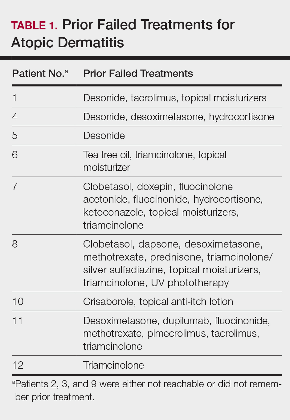
Inclusion criteria included men and women 18 years or older at baseline who had AD that was considered amenable to therapy with topical corticosteroids by the clinician and were able to comply with the study protocol (Figure). Written informed consent also was obtained from each patient. Women who were pregnant, breastfeeding, or unwilling to practice birth control during participation in the study were excluded. Other exclusion criteria included presence of a condition that in the opinion of the investigator would compromise the safety of the patient or quality of data as well as patients with no access to a telephone throughout the day. Patients diagnosed with conditions affecting adherence to treatment (eg, dementia, Alzheimer disease), those with a history of allergy or sensitivity to corticosteroids, and those with a history of drug hypersensitivity were excluded from the study.
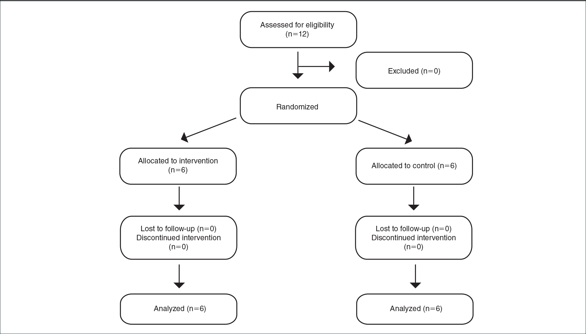
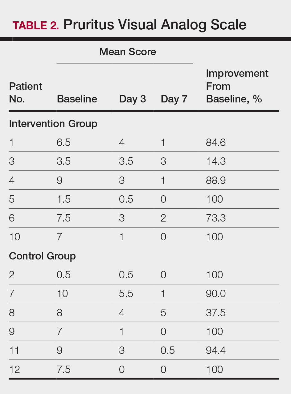
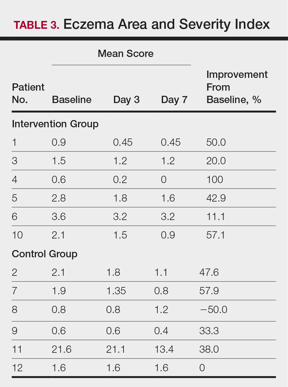
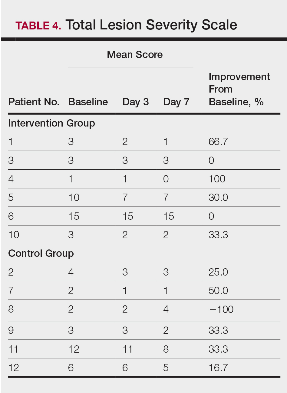
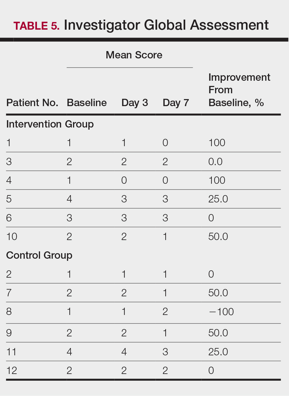
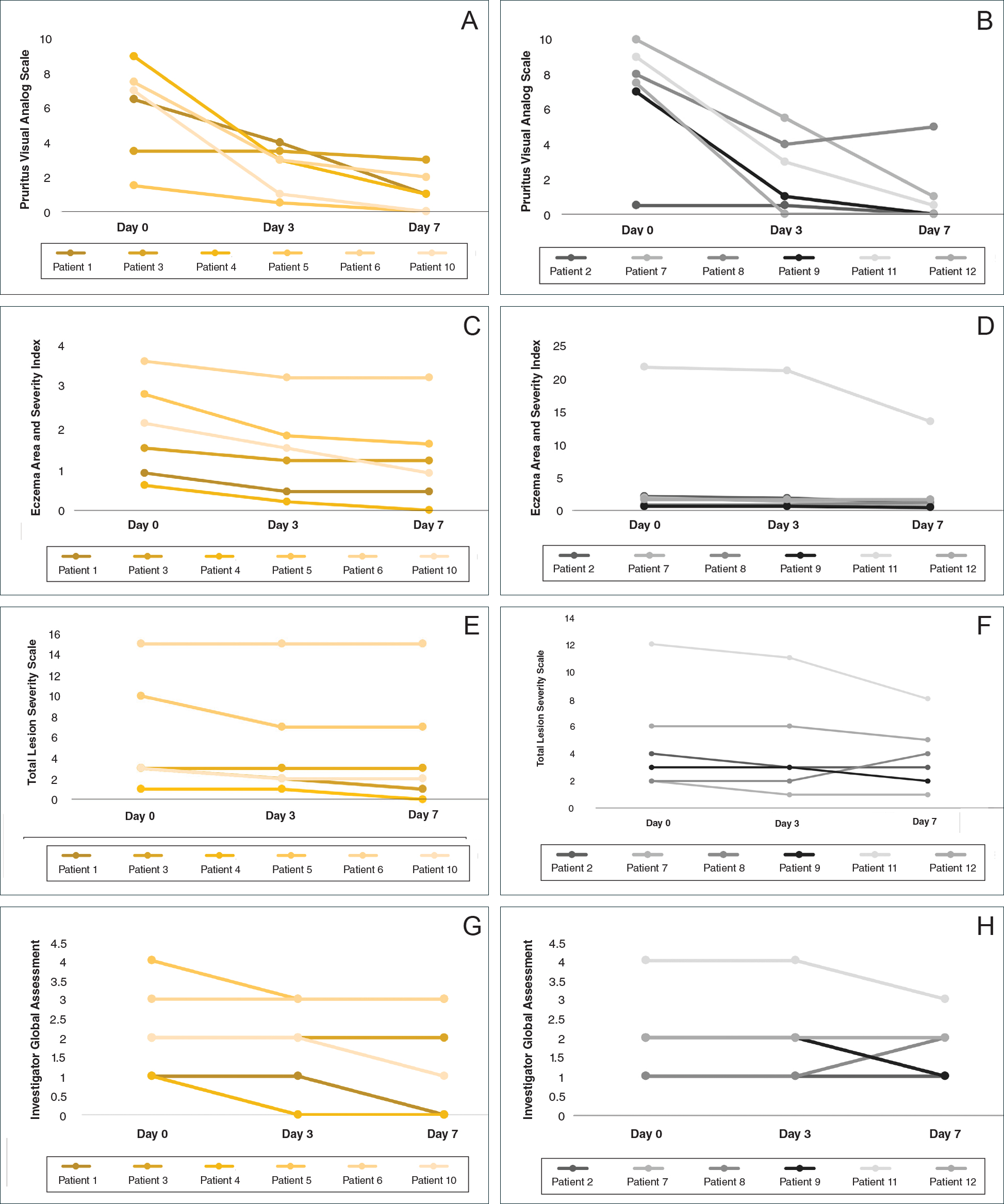
All 12 patients were treated with desoximetasone spray 0.25% for 7 days. Patients were instructed not to use other AD medications during the study period. At baseline, patients were randomized to receive either twice-daily telephone calls to discuss treatment adherence (intervention group) or no telephone calls (control) during the study period. Patients in both the intervention and control groups returned for evaluation on days 3 and 7. During these visits, disease severity was evaluated using the pruritus visual analog scale, Eczema Area and Severity Index (EASI), total lesion severity scale (TLSS), and investigator global assessment (IGA). Descriptive statistics were used to report the outcomes for each patient.
Results
Twelve AD patients who were previously unsuccessfully treated with topical corticosteroids were recruited for the study. Six patients were randomized to the intervention group and 6 were randomized to the control group. Fifty percent of patients were black, 50% were women, and the average age was 50.4 years. All 12 patients completed the study.
At the end of the study, most patients showed improvement in all evaluation parameters (eFigure). All 12 patients showed improvement in pruritus visual analog scores; 83.3% (10/12) showed improved EASI scores, 75.0% (9/12) showed improved TLSS scores, and 58.3% (7/12) showed improved IGA scores (Tables 2–5). Patients who received telephone calls in the intervention group showed greater improvement compared to those in the control group, except for pruritus; the mean reduction in pruritus was 76.9% in the intervention group versus 87.0% in the control group. The mean improvement in EASI score was 46.9% in the intervention group versus 21.1% in the control group. The mean improvement in TLSS score was 38.3% in the intervention group versus 9.7% in the control group. The mean improvement in IGA score was 45.8% in the intervention group versus 4.2% in the control group. Only one patient in the control group (patient 8) showed lower EASI, TLSS, and IGA scores at baseline.
Comment
Although topical corticosteroids are the mainstay for treatment of AD, many patients report treatment resistance after a period of a few doses or longer.6-9 There is strong evidence demonstrating rapid corticosteroid receptor downregulation in tissues after corticosteroid therapy, which is the accepted mechanism for tachyphylaxis, but the timing of this effect does not match up with clinical experiences. The physiologic significance of corticosteroid agonist-induced receptor downregulation is unknown and may not have any considerable effect on corticosteroid efficacy.3 A systematic review by Taheri et al3 on the development of resistance to topical corticosteroids proposed 2 theories for the underlying pathogenesis of tachyphylaxis: (1) long-term patient nonadherence, and (2) the initial maximal response during the first few weeks of therapy eventually plateaus. Because corticosteroids may plateau after a certain number of doses, natural disease flare-ups during this period may give the wrong impression of tachyphylaxis.10 The treatment “resistance” reported by the patients in our study may have been due to this plateau effect or to poor adherence.
Our finding that nearly all patients had rapid improvement of AD with the topical corticosteroid is not definitive proof but supports the notion that tachyphylaxis is largely mediated by poor adherence to treatment. Patients rapidly improved over the short study period. The short duration of treatment and multiple visits over the study period were designed to help ensure patient adherence. Rapid improvement in AD when topical corticosteroids are used should be expected, as AD patients have rapid improvement with application of topical corticosteroids in inpatient settings.11,12
Poor adherence to topical medication is common. In a Danish study, 99 of 322 patients (31%) did not redeem their AD prescriptions.13 In a single-center, 5-day, prospective study evaluating the use of fluocinonide cream 0.1% for treatment of children and adults with AD, the median percentage of prescribed doses taken was 40%, according to objective electronic monitors, even though patients reported 100% adherence in their medication diaries.Better adherence was seen on day 1 of treatment in which 66.6% (6/9) of patients adhered to their treatment strategy versus day 5 in which only 11.1% (1/9) of patients used their medication.1
Topical corticosteroids are safe and efficacious if used appropriately; however, patients commonly express fear and anxiety about using them. Topical corticosteroid phobia may stem from a misconception that these products carry the same adverse effects as their oral and systemic counterparts, which may be perpetuated by the media.1 Of 200 dermatology patients surveyed, 72.5% expressed concern about using topical corticosteroids on themselves or their children’s skin, and 24% of these patients stated they were noncompliant with their medication because of these worries. Almost 50% of patients requested prescriptions for corticosteroid-sparing medications such as tacrolimus.1 Patient education is important to help ensure treatment adherence. Other factors that can affect treatment adherence include forgetfulness; the chronic nature of AD; the need for ongoing application of topical treatments; prohibitive costs of some topical agents; and complexities in coordinating school, work, and family plans with the treatment regimen.2
We attempted to ensure good treatment adherence in our study by calling the patients in the intervention group twice daily. The mean improvement in EASI, TLSS, and IGA scores was higher in the intervention group versus the control group, which suggests that patient reminders have at least some benefit. Because AD treatment resistance appears more closely tied to nonadherence rather than loss of medication efficacy, it seems prudent to focus on interventions that would improve treatment adherence; however, such interventions generally are not well tested. Recommended interventions have included educating patients about the side effects of topical corticosteroids, avoiding use of medical jargon, and taking patient vehicle preference into account when prescribing treatments.8 Patients should be scheduled for a return visit within 1 to 2 weeks, as early return visits can augment treatment adherence.14 At the return visit, there can be a more detailed discussion of long-term management and side effects.8
Limitations of our study included a small sample size and brief treatment duration. Even though the patients had previously reported treatment failure with topical corticosteroids, all demonstrated improvement in only 1 week with a potent topical corticosteroid. The treatment resistance that initially was reported likely was due to poor adherence, but it is possible for AD patients to be resistant to treatment with topical corticosteroids due to allergic contact dermatitis. Patients could theoretically be allergic to components of the vehicle used in topical corticosteroids, which could aggravate their dermatitis; however, this effect seems unlikely in our patient population, as all the patients in our study showed improvement following treatment. Another study limitation was that adherence was not measured. The frequent follow-up visits were designed to encourage treatment adherence, but adherence was not specifically assessed. Although patients were encouraged to only use the desoximetasone spray during the study, it is not known whether patients used other products.
Conclusion
Some AD patients exhibit apparent decreased efficacy of topical corticosteroids over time, but this tachyphylaxis phenomenon is more likely due to poor treatment adherence than to loss of corticosteroid responsiveness. In our study, AD patients who reported treatment failure with topical corticosteroids improved rapidly with topical corticosteroids under conditions designed to promote good adherence to treatment. The majority of patients improved in all 4 parameters used for evaluating disease severity, with 100% of patients reporting improvement in pruritus. Intervention to improve treatment adherence may lead to better health outcomes. When AD appears resistant to topical corticosteroids, addressing adherence issues may be critical.
- Patel NU, D’Ambra V, Feldman SR. Increasing adherence with topical agents for atopic dermatitis. Am J Clin Dermatol. 2017;18:323-332.
- Mooney E, Rademaker M, Dailey R, et al. Adverse effects of topical corticosteroids in paediatric eczema: Australasian consensus statement. Australas J Dermatol. 2015;56:241-251.
- Taheri A, Cantrell J, Feldman SR. Tachyphylaxis to topical glucocorticoids; what is the evidence? Dermatol Online J. 2013;19:18954.
- Miller JJ, Roling D, Margolis D, et al. Failure to demonstrate therapeutic tachyphylaxis to topically applied steroids in patients with psoriasis. J Am Acad Dermatol. 1999;41:546-549.
- Smith SD, Harris V, Lee A, et al. General practitioners knowledge about use of topical corticosteroids in paediatric atopic dermatitis in Australia. Aust Fam Physician. 2017;46:335-340.
- Sathishkumar D, Moss C. Topical therapy in atopic dermatitis in children. Indian J Dermatol. 2016;61:656-661.
- Reitamo S, Remitz A. Topical agents for atopic dermatitis. In: Bieber T, ed. Advances in the Management of Atopic Dermatitis. London, United Kingdom: Future Medicine Ltd; 2013:62-72.
- Krejci-Manwaring J, Tusa MG, Carroll C, et al. Stealth monitoring of adherence to topical medication: adherence is very poor in children with atopic dermatitis. J Am Acad Dermatol. 2007;56:211-216.
- Fukaya M. Cortisol homeostasis in the epidermis is influenced by topical corticosteroids in patients with atopic dermatitis. Indian J Dermatol. 2017;62:440.
- Mehta AB, Nadkarni NJ, Patil SP, et al. Topical corticosteroids in dermatology. Indian J Dermatol Venereol Leprol. 2016;82:371-378.
- van der Schaft J, Keijzer WW, Sanders KJ, et al. Is there an additional value of inpatient treatment for patients with atopic dermatitis? Acta Derm Venereol. 2016;96:797-801.
- Dabade TS, Davis DM, Wetter DA, et al. Wet dressing therapy in conjunction with topical corticosteroids is effective for rapid control of severe pediatric atopic dermatitis: experience with 218 patients over 30 years at Mayo Clinic. J Am Acad Dermatol. 2011;67:100-106.
- Storm A, Andersen SE, Benfeldt E, et al. One in 3 prescriptions are never redeemed: primary nonadherence in an outpatient clinic. J Am Acad Dermatol. 2008;59:27-33.
- Sagransky MJ, Yentzer BA, Williams LL, et al. A randomized controlled pilot study of the effects of an extra office visit on adherence and outcomes in atopic dermatitis. Arch Dermatol. 2010;146:1428-1430.
Atopic dermatitis (AD) is most often treated with mid-potency topical corticosteroids.1,2 Although this option is effective, not all patients respond to treatment, and those who do may lose efficacy over time, a phenomenon known as tachyphylaxis. The pathophysiology of tachyphylaxis to topical corticosteroids has been ascribed to loss of corticosteroid receptor function,3 but the evidence is weak.3,4 Patients with severe treatment-resistant AD improve when treated with mid-potency topical steroids in an inpatient setting; therefore, treatment resistance to topical corticosteroids may be largely due to poor adherence.5
Patients with treatment-resistant AD generally improve when treated with topical corticosteroids under conditions designed to promote treatment adherence, but this improvement often is reported for study groups, not individual patients. Focusing on group data may not give a clear picture of what is happening at the individual level. In this study, we evaluated changes at an individual level to determine how frequently AD patients who were previously treated with topical corticosteroids unsuccessfully would respond to desoximetasone spray 0.25% under conditions designed to promote good adherence over a 7-day period.
Methods
This open-label, randomized, single-center clinical study included 12 patients with AD who were previously unsuccessfully treated with topical corticosteroids in the Department of Dermatology at Wake Forest Baptist Medical Center (Winston-Salem, North Carolina)(Table 1). The study was approved by the local institutional review board.
Inclusion criteria included men and women 18 years or older at baseline who had AD that was considered amenable to therapy with topical corticosteroids by the clinician and were able to comply with the study protocol (Figure). Written informed consent also was obtained from each patient. Women who were pregnant, breastfeeding, or unwilling to practice birth control during participation in the study were excluded. Other exclusion criteria included presence of a condition that in the opinion of the investigator would compromise the safety of the patient or quality of data as well as patients with no access to a telephone throughout the day. Patients diagnosed with conditions affecting adherence to treatment (eg, dementia, Alzheimer disease), those with a history of allergy or sensitivity to corticosteroids, and those with a history of drug hypersensitivity were excluded from the study.
All 12 patients were treated with desoximetasone spray 0.25% for 7 days. Patients were instructed not to use other AD medications during the study period. At baseline, patients were randomized to receive either twice-daily telephone calls to discuss treatment adherence (intervention group) or no telephone calls (control) during the study period. Patients in both the intervention and control groups returned for evaluation on days 3 and 7. During these visits, disease severity was evaluated using the pruritus visual analog scale, Eczema Area and Severity Index (EASI), total lesion severity scale (TLSS), and investigator global assessment (IGA). Descriptive statistics were used to report the outcomes for each patient.
Results
Twelve AD patients who were previously unsuccessfully treated with topical corticosteroids were recruited for the study. Six patients were randomized to the intervention group and 6 were randomized to the control group. Fifty percent of patients were black, 50% were women, and the average age was 50.4 years. All 12 patients completed the study.
At the end of the study, most patients showed improvement in all evaluation parameters (eFigure). All 12 patients showed improvement in pruritus visual analog scores; 83.3% (10/12) showed improved EASI scores, 75.0% (9/12) showed improved TLSS scores, and 58.3% (7/12) showed improved IGA scores (Tables 2–5). Patients who received telephone calls in the intervention group showed greater improvement compared to those in the control group, except for pruritus; the mean reduction in pruritus was 76.9% in the intervention group versus 87.0% in the control group. The mean improvement in EASI score was 46.9% in the intervention group versus 21.1% in the control group. The mean improvement in TLSS score was 38.3% in the intervention group versus 9.7% in the control group. The mean improvement in IGA score was 45.8% in the intervention group versus 4.2% in the control group. Only one patient in the control group (patient 8) showed lower EASI, TLSS, and IGA scores at baseline.
Comment
Although topical corticosteroids are the mainstay for treatment of AD, many patients report treatment resistance after a period of a few doses or longer.6-9 There is strong evidence demonstrating rapid corticosteroid receptor downregulation in tissues after corticosteroid therapy, which is the accepted mechanism for tachyphylaxis, but the timing of this effect does not match up with clinical experiences. The physiologic significance of corticosteroid agonist-induced receptor downregulation is unknown and may not have any considerable effect on corticosteroid efficacy.3 A systematic review by Taheri et al3 on the development of resistance to topical corticosteroids proposed 2 theories for the underlying pathogenesis of tachyphylaxis: (1) long-term patient nonadherence, and (2) the initial maximal response during the first few weeks of therapy eventually plateaus. Because corticosteroids may plateau after a certain number of doses, natural disease flare-ups during this period may give the wrong impression of tachyphylaxis.10 The treatment “resistance” reported by the patients in our study may have been due to this plateau effect or to poor adherence.
Our finding that nearly all patients had rapid improvement of AD with the topical corticosteroid is not definitive proof but supports the notion that tachyphylaxis is largely mediated by poor adherence to treatment. Patients rapidly improved over the short study period. The short duration of treatment and multiple visits over the study period were designed to help ensure patient adherence. Rapid improvement in AD when topical corticosteroids are used should be expected, as AD patients have rapid improvement with application of topical corticosteroids in inpatient settings.11,12
Poor adherence to topical medication is common. In a Danish study, 99 of 322 patients (31%) did not redeem their AD prescriptions.13 In a single-center, 5-day, prospective study evaluating the use of fluocinonide cream 0.1% for treatment of children and adults with AD, the median percentage of prescribed doses taken was 40%, according to objective electronic monitors, even though patients reported 100% adherence in their medication diaries.Better adherence was seen on day 1 of treatment in which 66.6% (6/9) of patients adhered to their treatment strategy versus day 5 in which only 11.1% (1/9) of patients used their medication.1
Topical corticosteroids are safe and efficacious if used appropriately; however, patients commonly express fear and anxiety about using them. Topical corticosteroid phobia may stem from a misconception that these products carry the same adverse effects as their oral and systemic counterparts, which may be perpetuated by the media.1 Of 200 dermatology patients surveyed, 72.5% expressed concern about using topical corticosteroids on themselves or their children’s skin, and 24% of these patients stated they were noncompliant with their medication because of these worries. Almost 50% of patients requested prescriptions for corticosteroid-sparing medications such as tacrolimus.1 Patient education is important to help ensure treatment adherence. Other factors that can affect treatment adherence include forgetfulness; the chronic nature of AD; the need for ongoing application of topical treatments; prohibitive costs of some topical agents; and complexities in coordinating school, work, and family plans with the treatment regimen.2
We attempted to ensure good treatment adherence in our study by calling the patients in the intervention group twice daily. The mean improvement in EASI, TLSS, and IGA scores was higher in the intervention group versus the control group, which suggests that patient reminders have at least some benefit. Because AD treatment resistance appears more closely tied to nonadherence rather than loss of medication efficacy, it seems prudent to focus on interventions that would improve treatment adherence; however, such interventions generally are not well tested. Recommended interventions have included educating patients about the side effects of topical corticosteroids, avoiding use of medical jargon, and taking patient vehicle preference into account when prescribing treatments.8 Patients should be scheduled for a return visit within 1 to 2 weeks, as early return visits can augment treatment adherence.14 At the return visit, there can be a more detailed discussion of long-term management and side effects.8
Limitations of our study included a small sample size and brief treatment duration. Even though the patients had previously reported treatment failure with topical corticosteroids, all demonstrated improvement in only 1 week with a potent topical corticosteroid. The treatment resistance that initially was reported likely was due to poor adherence, but it is possible for AD patients to be resistant to treatment with topical corticosteroids due to allergic contact dermatitis. Patients could theoretically be allergic to components of the vehicle used in topical corticosteroids, which could aggravate their dermatitis; however, this effect seems unlikely in our patient population, as all the patients in our study showed improvement following treatment. Another study limitation was that adherence was not measured. The frequent follow-up visits were designed to encourage treatment adherence, but adherence was not specifically assessed. Although patients were encouraged to only use the desoximetasone spray during the study, it is not known whether patients used other products.
Conclusion
Some AD patients exhibit apparent decreased efficacy of topical corticosteroids over time, but this tachyphylaxis phenomenon is more likely due to poor treatment adherence than to loss of corticosteroid responsiveness. In our study, AD patients who reported treatment failure with topical corticosteroids improved rapidly with topical corticosteroids under conditions designed to promote good adherence to treatment. The majority of patients improved in all 4 parameters used for evaluating disease severity, with 100% of patients reporting improvement in pruritus. Intervention to improve treatment adherence may lead to better health outcomes. When AD appears resistant to topical corticosteroids, addressing adherence issues may be critical.
- Patel NU, D’Ambra V, Feldman SR. Increasing adherence with topical agents for atopic dermatitis. Am J Clin Dermatol. 2017;18:323-332.
- Mooney E, Rademaker M, Dailey R, et al. Adverse effects of topical corticosteroids in paediatric eczema: Australasian consensus statement. Australas J Dermatol. 2015;56:241-251.
- Taheri A, Cantrell J, Feldman SR. Tachyphylaxis to topical glucocorticoids; what is the evidence? Dermatol Online J. 2013;19:18954.
- Miller JJ, Roling D, Margolis D, et al. Failure to demonstrate therapeutic tachyphylaxis to topically applied steroids in patients with psoriasis. J Am Acad Dermatol. 1999;41:546-549.
- Smith SD, Harris V, Lee A, et al. General practitioners knowledge about use of topical corticosteroids in paediatric atopic dermatitis in Australia. Aust Fam Physician. 2017;46:335-340.
- Sathishkumar D, Moss C. Topical therapy in atopic dermatitis in children. Indian J Dermatol. 2016;61:656-661.
- Reitamo S, Remitz A. Topical agents for atopic dermatitis. In: Bieber T, ed. Advances in the Management of Atopic Dermatitis. London, United Kingdom: Future Medicine Ltd; 2013:62-72.
- Krejci-Manwaring J, Tusa MG, Carroll C, et al. Stealth monitoring of adherence to topical medication: adherence is very poor in children with atopic dermatitis. J Am Acad Dermatol. 2007;56:211-216.
- Fukaya M. Cortisol homeostasis in the epidermis is influenced by topical corticosteroids in patients with atopic dermatitis. Indian J Dermatol. 2017;62:440.
- Mehta AB, Nadkarni NJ, Patil SP, et al. Topical corticosteroids in dermatology. Indian J Dermatol Venereol Leprol. 2016;82:371-378.
- van der Schaft J, Keijzer WW, Sanders KJ, et al. Is there an additional value of inpatient treatment for patients with atopic dermatitis? Acta Derm Venereol. 2016;96:797-801.
- Dabade TS, Davis DM, Wetter DA, et al. Wet dressing therapy in conjunction with topical corticosteroids is effective for rapid control of severe pediatric atopic dermatitis: experience with 218 patients over 30 years at Mayo Clinic. J Am Acad Dermatol. 2011;67:100-106.
- Storm A, Andersen SE, Benfeldt E, et al. One in 3 prescriptions are never redeemed: primary nonadherence in an outpatient clinic. J Am Acad Dermatol. 2008;59:27-33.
- Sagransky MJ, Yentzer BA, Williams LL, et al. A randomized controlled pilot study of the effects of an extra office visit on adherence and outcomes in atopic dermatitis. Arch Dermatol. 2010;146:1428-1430.
Practice Points
- Mid-potency corticosteroids are the first-line treatment of atopic dermatitis (AD).
- Atopic dermatitis may fail to respond to topical corticosteroids initially or lose response over time, a phenomenon known as tachyphylaxis.
- Nonadherence to medication is the most likely cause of treatment resistance in patients with AD.
Molluscum Contagiosum Virus Infection Can Trigger Atopic Dermatitis Disease Onset or Flare
Molluscum contagiosum virus (MCV) is a common pediatric viral infection of the skin and/or mucous membranes.1 It has been noted in increasingly younger patient populations, ranging from congenital cases resulting from perinatal/vertical transmission to transmission from cobathing and pool usage.2,3
An association between MCV infection and atopic dermatitis (AD) has been reported to be caused by a predisposition to prolonged and severe cutaneous viral infections.4 However, the exact nature of the relationship between MCV and AD is unknown.
The purpose of this study was to identify pediatric patients with AD onset or flare of AD triggered by MCV infection as well as to characterize the setting under which MCV may trigger AD onset or flares in children.
Methods
Medical records for 50 children with prior or current MCV infection who presented sequentially to an outpatient pediatric dermatology practice over a 1-month period were identified. Institutional review board approval was obtained.
Results
The age range of the 50 patients with MCV infection was 1 to 13 years, with an average age of 3.6 years at the onset of infection (reported by parents/guardians) and 4.5 years at presentation to the pediatric dermatology office (Table 1).
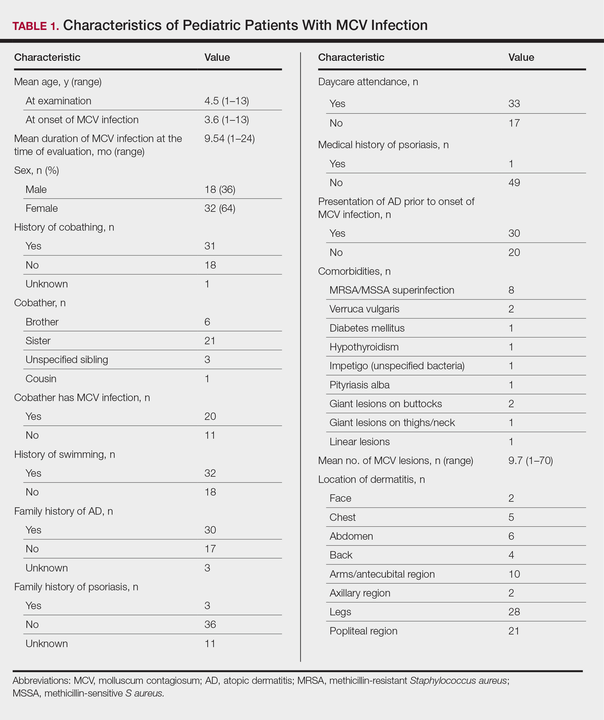
The role of cobathing is unknown; however, 62% (31/50) of patients previously or currently cobathed at home, suggesting it may be a risk factor for MCV infection. An association of MCV lesions in the popliteal region trended toward being more likely with cobathing, but the association was not statistically significant.
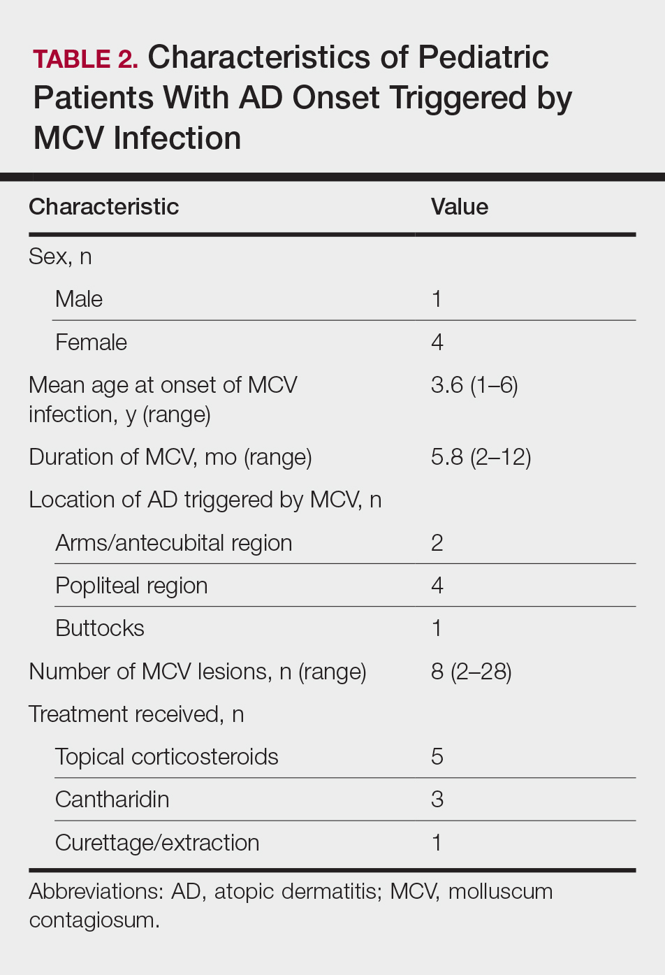
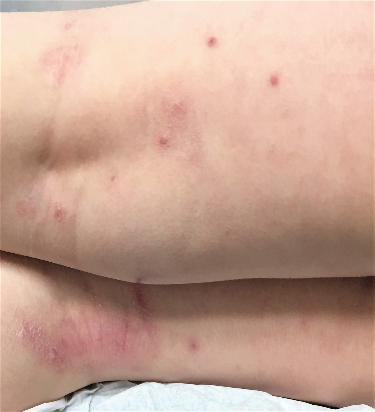
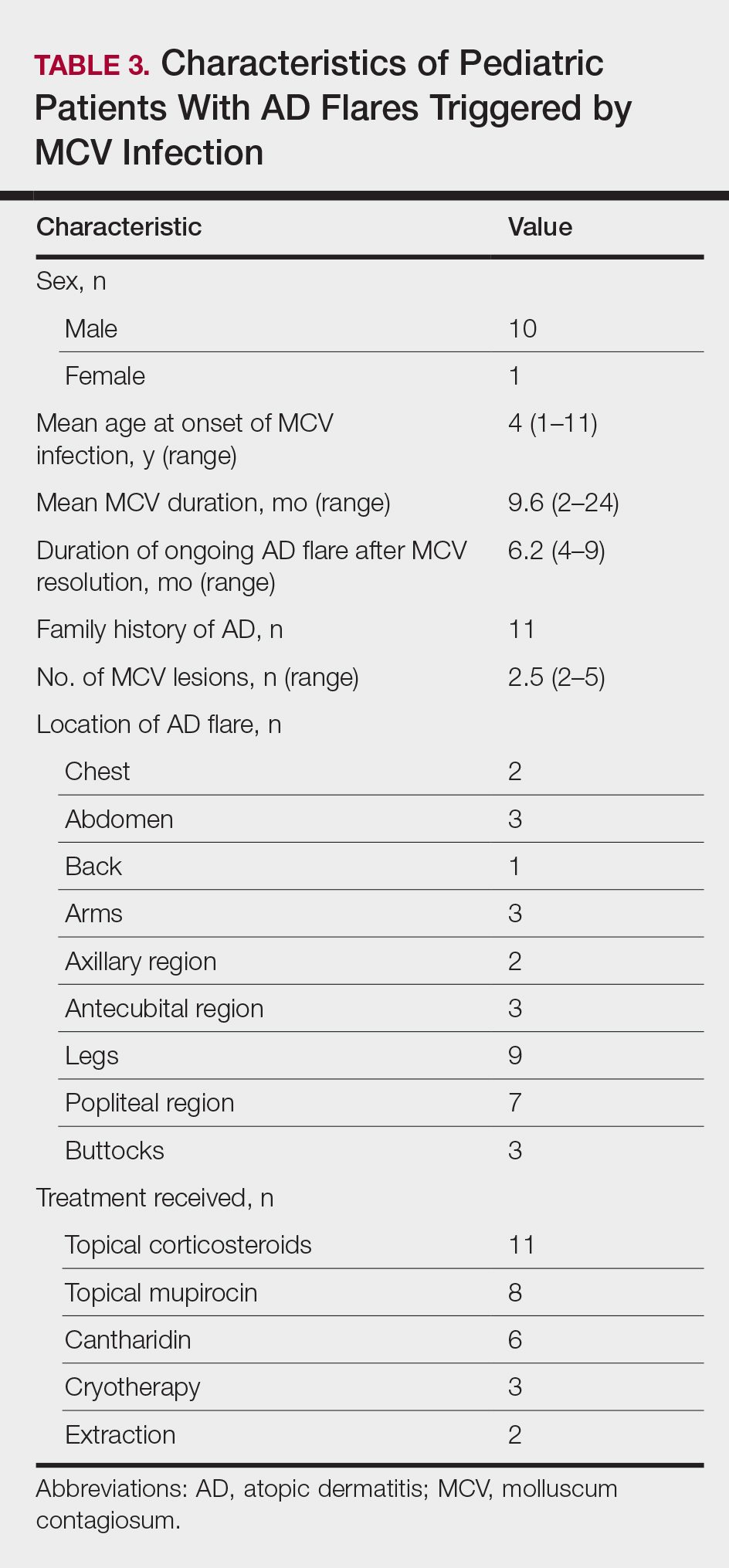
Children with AD onset triggered by MCV infection statistically were more likely to have flexural localization of MCV and AD lesions and were statistically more likely to have a family history of AD (P<.04)(Table 2). Children with AD flares triggered by MCV infection were more likely to have MCV and AD lesions of the popliteal region and legs (P<.05)(Figure) and family history of AD (P<.04)(Table 3). Location of MCV lesions on the upper and lower extremities, buttocks, and genitalia were more likely to be associated with presence of any dermatitis than facial and/or truncal lesions (P<.05). Treatment of the MCV infection did not appear to impact the course of AD when present, but prospective interventions would be needed to assess this issue.
Superinfection with methicillin-resistant and methicillin-sensitive Staphylococcus aureus as well as atypical giant lesions of the intertriginous neck, inner thighs, and buttocks also were noted, but AD was uncommon in these cases. Given the limited number of cases, statistical significance could not be assessed.
Comment
Cutaneous infections with Malassezia have been postulated to trigger AD in infancy,1 while systemic viral infections such as varicella-zoster virus may be protective against AD when acquired in younger children.7 It appears that MCV infection in young children (eg, 3 years or younger) with specific localization to the flexural areas has the potential to trigger AD in susceptible hosts. Larger studies are needed to chart the long-term disease course of AD in these children. Due to the small size of this study, it is unclear if the rise of MCV infections since the 1980s has contributed to increased AD.8 Susceptible children appear to have a family history of AD and localization of MCV lesions on the legs, buttocks, and antecubital region. Atopic dermatitis risk appears to be highest when MCV lesions are localized to intertriginous or flexural locations.
In addition to triggering the onset of AD, MCV infection also can trigger persistent flaring of AD, especially in the popliteal region and legs. Atopic dermatitis flares can occur at any age, but they appear to cluster in preschoolers and typically are not prevented by AD or MCV treatments; however, randomized trials are needed to identify if early intervention of MCV has a preventive benefit on AD onset or flares, and longer-term observation is needed to identify true disease course modification. Reduction of the number of MCV lesions previously has been demonstrated with institution of topical corticosteroid therapy.6 Therefore, institution of atopic skin care generally is advisable in the setting of MCV infection. Future studies should address the potential use of interventions to prevent the triggering of AD onset or flares in the setting of MCV infection in children.5
- Brown J, Janniger CK, Schwartz RA, et al. Childhood molluscum contagiosum. Int J Dermatol. 2006;45:93-99.
- Connell CO, Oranje A, Van Gysel D, et al. Congenital molluscum contagiosum: report of four cases and review of the literature. Pediatr Dermatol. 2008;25:553-556.
- Luke JD, Silverberg NB. Vertically transmitted molluscum contagiosum infection. Pediatrics. 2010;125:E423-E425.
- Olsen JR, Piguet V, Gallacher J, et al. Molluscum contagiosum and associations with atopic eczema in children: a retrospective longitudinal study in primary care. Br J Gen Pract. 2016;66:E53-E58.
- Basdag H, Rainer BM, Cohen BA. Molluscum contagiosum: to treat or not to treat? experience with 170 children in an outpatient clinic setting in the northeastern United States. Pediatr Dermatol. 2015;32:353-357.
- Berger EM, Orlow SJ, Patel RR, et al. Experience with molluscum contagiosum and associated inflammatory reactions in a pediatric dermatology practice: the bump that rashes. Arch Dermatol. 2012;148:1257-1264.
- Silverberg JI, Norowitz KB, Kleiman E, et al. Association between varicella zoster virus infection and atopic dermatitis in early and late childhood: a case-control study. J Allergy Clin Immunol. 2010;126:300-305.
- Oriel JD. The increase in molluscum contagiosum. Br Med J (Clin Res Ed). 1987;294:74.
Molluscum contagiosum virus (MCV) is a common pediatric viral infection of the skin and/or mucous membranes.1 It has been noted in increasingly younger patient populations, ranging from congenital cases resulting from perinatal/vertical transmission to transmission from cobathing and pool usage.2,3
An association between MCV infection and atopic dermatitis (AD) has been reported to be caused by a predisposition to prolonged and severe cutaneous viral infections.4 However, the exact nature of the relationship between MCV and AD is unknown.
The purpose of this study was to identify pediatric patients with AD onset or flare of AD triggered by MCV infection as well as to characterize the setting under which MCV may trigger AD onset or flares in children.
Methods
Medical records for 50 children with prior or current MCV infection who presented sequentially to an outpatient pediatric dermatology practice over a 1-month period were identified. Institutional review board approval was obtained.
Results
The age range of the 50 patients with MCV infection was 1 to 13 years, with an average age of 3.6 years at the onset of infection (reported by parents/guardians) and 4.5 years at presentation to the pediatric dermatology office (Table 1).
The role of cobathing is unknown; however, 62% (31/50) of patients previously or currently cobathed at home, suggesting it may be a risk factor for MCV infection. An association of MCV lesions in the popliteal region trended toward being more likely with cobathing, but the association was not statistically significant.
Children with AD onset triggered by MCV infection statistically were more likely to have flexural localization of MCV and AD lesions and were statistically more likely to have a family history of AD (P<.04)(Table 2). Children with AD flares triggered by MCV infection were more likely to have MCV and AD lesions of the popliteal region and legs (P<.05)(Figure) and family history of AD (P<.04)(Table 3). Location of MCV lesions on the upper and lower extremities, buttocks, and genitalia were more likely to be associated with presence of any dermatitis than facial and/or truncal lesions (P<.05). Treatment of the MCV infection did not appear to impact the course of AD when present, but prospective interventions would be needed to assess this issue.
Superinfection with methicillin-resistant and methicillin-sensitive Staphylococcus aureus as well as atypical giant lesions of the intertriginous neck, inner thighs, and buttocks also were noted, but AD was uncommon in these cases. Given the limited number of cases, statistical significance could not be assessed.
Comment
Cutaneous infections with Malassezia have been postulated to trigger AD in infancy,1 while systemic viral infections such as varicella-zoster virus may be protective against AD when acquired in younger children.7 It appears that MCV infection in young children (eg, 3 years or younger) with specific localization to the flexural areas has the potential to trigger AD in susceptible hosts. Larger studies are needed to chart the long-term disease course of AD in these children. Due to the small size of this study, it is unclear if the rise of MCV infections since the 1980s has contributed to increased AD.8 Susceptible children appear to have a family history of AD and localization of MCV lesions on the legs, buttocks, and antecubital region. Atopic dermatitis risk appears to be highest when MCV lesions are localized to intertriginous or flexural locations.
In addition to triggering the onset of AD, MCV infection also can trigger persistent flaring of AD, especially in the popliteal region and legs. Atopic dermatitis flares can occur at any age, but they appear to cluster in preschoolers and typically are not prevented by AD or MCV treatments; however, randomized trials are needed to identify if early intervention of MCV has a preventive benefit on AD onset or flares, and longer-term observation is needed to identify true disease course modification. Reduction of the number of MCV lesions previously has been demonstrated with institution of topical corticosteroid therapy.6 Therefore, institution of atopic skin care generally is advisable in the setting of MCV infection. Future studies should address the potential use of interventions to prevent the triggering of AD onset or flares in the setting of MCV infection in children.5
- Brown J, Janniger CK, Schwartz RA, et al. Childhood molluscum contagiosum. Int J Dermatol. 2006;45:93-99.
- Connell CO, Oranje A, Van Gysel D, et al. Congenital molluscum contagiosum: report of four cases and review of the literature. Pediatr Dermatol. 2008;25:553-556.
- Luke JD, Silverberg NB. Vertically transmitted molluscum contagiosum infection. Pediatrics. 2010;125:E423-E425.
- Olsen JR, Piguet V, Gallacher J, et al. Molluscum contagiosum and associations with atopic eczema in children: a retrospective longitudinal study in primary care. Br J Gen Pract. 2016;66:E53-E58.
- Basdag H, Rainer BM, Cohen BA. Molluscum contagiosum: to treat or not to treat? experience with 170 children in an outpatient clinic setting in the northeastern United States. Pediatr Dermatol. 2015;32:353-357.
- Berger EM, Orlow SJ, Patel RR, et al. Experience with molluscum contagiosum and associated inflammatory reactions in a pediatric dermatology practice: the bump that rashes. Arch Dermatol. 2012;148:1257-1264.
- Silverberg JI, Norowitz KB, Kleiman E, et al. Association between varicella zoster virus infection and atopic dermatitis in early and late childhood: a case-control study. J Allergy Clin Immunol. 2010;126:300-305.
- Oriel JD. The increase in molluscum contagiosum. Br Med J (Clin Res Ed). 1987;294:74.
Practice Points
- Molluscum contagiosum virus (MCV) infection appears to aggravate atopic dermatitis (AD) symptoms in a subset of pediatric patients.
- In susceptible children, the first onset of AD symptoms can occur during the course of MCV infection.
Headless Compression Screw Fixation of Vertical Medial Malleolus Fractures is Superior to Unicortical Screw Fixation
ABSTRACT
This study is the first biomechanical research of headless compression screws for fixation of vertical shear fractures of the medial malleolus, a promising alternative that potentially offers several advantages for fixation.
Vertical shear fractures were simulated by osteotomies in 20 synthetic distal tibiae. Models were randomly assigned to fixation with either 2 parallel cancellous screws or 2 parallel Acutrak 2 headless compression screws (Acumed). Specimens were subjected to offset axial loading to simulate supination-adduction loading and tracked using high-resolution video.
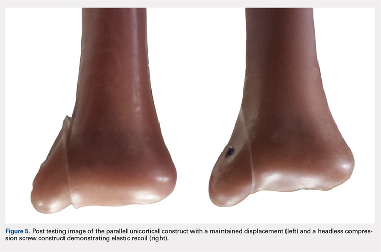
The headless compression screw construct was significantly stiffer (P < .0001) (360 ± 131 N/mm) than the partially threaded cancellous screws (180 ± 48 N/mm) and demonstrated a significantly increased (P < .0001) mean load to clinical failure (719 ± 91 N vs 343 ± 83 N). When specimens were displaced to 6 mm and allowed to relax, the headless compression screw constructs demonstrated an elastic recoil and were reduced to the pretesting fragment alignment, whereas the parallel cancellous screw constructs remained displaced.
Along with the headless design that may decrease soft tissue irritation, the increased stiffness and elastic recoil of the headless compression screw construct offers improved fixation of medial malleolus vertical shear fractures over the traditional methods.
Continue to: Headless compressions screws...
Headless compressions screws are cannulated tapered titanium screws with variable thread pitch angle, allowing a fully threaded screw to apply compression along its entire length. These screws have been most commonly used for scaphoid fractures1 but have also been studied in fractures of small bones, such as capitellum, midfoot, and talar neck,2-4 and arthrodesis in the foot, ankle, and hand.5-7 Headless compression screws have been found to produce equivalent fragment compression to partially threaded cancellous screws while allowing less fragment displacement.8,9 The lack of a head may decrease soft tissue irritation compared with the partially threaded cancellous screws. Finally, headless compression screws are independent of cortical integrity, as the entire length of the screw features a wide thread diameter to capture cancellous bone in the proximal fragment, unlike partially threaded cancellous screws, which only possess a thread purchase in the distal fragment and depend on an intact cortex.
Vertical shear fractures of the medial malleolus occur through the supination-adduction of the talus exerted onto the articular surface of the medial malleolus.10 Optimal fixation of these fractures must be sufficient to maintain stable anatomic reduction of the ankle joint articular surface, allowing early range of motion, maintaining congruency of the ankle joint, and decreasing the risk of future post-traumatic arthritis to maximize functional outcome.11
A wide variety of techniques are available for fixation of these fractures, including various configurations of cortical screws, cancellous screws, tension bands, and antiglide plates. Clinically, 2 parallel 4.0-mm partially threaded cancellous screws are most often used. Limited evidence indicates that headless compression screws may be a viable option for fixation of medial malleolus fractures. One case reports the use of a headless compression screw for a horizontal medial malleolar fracture,12 and a small retrospective case series that used headless compression screws for all medial malleolar fractures showed satisfactory outcomes, a high union rate, and low patient-reported pain.13
We evaluate the stiffness, force to 2-mm displacement of the joint surface, and elastic properties of these 2 different constructs in vertical medial malleolar fractures in synthetic distal tibiae. We hypothesize that the parallel headless compression screw fixation will be stiffer and require more force to 2-mm displacement than parallel unicortical cancellous screw fixation.
MATERIALS AND METHODS
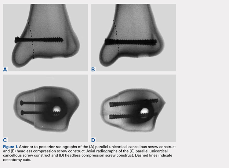
Identical vertical osteotomies (17.5 mm) were made from the medial border of the medial malleolus using a custom jig in 20 left 4th-generation composite synthetic distal tibiae (Sawbones, Pacific Research Labs; Model No. 3401) to simulate an Orthopaedic Trauma Association type 44-A2.3 fracture. The tibiae were then cut 18 cm from the tibial plafond and randomized to 2 fixation groups (n = 10 specimens for each group): parallel unicortical screw fixation or parallel unicortical headless compression screw fixation (Figures 1A-1D). Custom polymethylmethacrylate jigs were used to reproducibly drill identical holes with a 3.2-mm drill for the parallel unicortical screw construct and the drill bits provided by the Acutrak 2 Headless Compression Screw System (Acumed). The parallel unicortical screw construct consisted of 2 parallel 4.0-mm-diameter, 40-mm partially threaded cancellous screws (Depuy Synthes), and the headless compression fixation construct consisted of 2 parallel 4.7-mm-diameter, 45-mm titanium Acutrak 2 screws parallel to each other in the transverse plane. The Acutrak screws were placed per manufacturer instructions by first drilling with the Acutrak 2-4.7 Long Drill bit (Acumed), followed by the Acutrak 2-4.7 Profile Drill bit for the near cortex.
Continue to: Specimens...
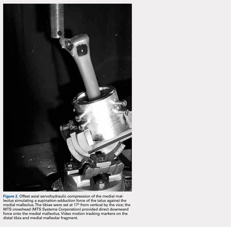
Specimens were fixed to the base of a servohydraulic testing machine (Model 809, MTS Systems Corporation) with an axial-torsional load transducer (Model No. 662.20-01; Axial capacity of 250 kg, torsional capacity 2.88 kg-m; MTS Systems Corporation). The specimens were set in a vice tilted at 17° in the coronal plane to allow the MTS crosshead to apply an offset axial load simulating supination-adduction loading, which has been described previously (Figure 2).14,15 Load was applied to the inferolateral articular surface of the medial malleolus at 1 mm/s to a crosshead displacement of 6 mm and then cycled back to 0 mm. Load and axial displacement were measured at 60 Hz. The markers on the distal tibia and medial malleolus fracture fragment were tracked using high-resolution video (Fastcam PCI, Photron USA Inc). The motion of the video markers was determined using digitization and motion analysis software (Motus 9, Vicon).
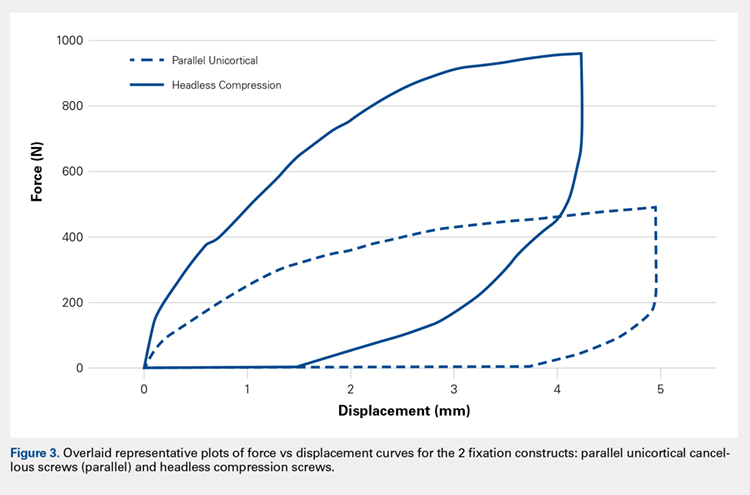
Stiffness was calculated as the slope of the linear portion of the load-displacement curve over a range of 0.5 to 2.0 mm (Figure 3) and reported as mean (standard deviation). The force at 2 mm of fragment displacement was defined as a clinical failure.16,17 Student’s t test was used to determine the difference in construct stiffness and force for 2 mm displacement of the 2 groups. Significance was defined as P < .05. Institutional Review Board approval was not required for this study.
RESULTS
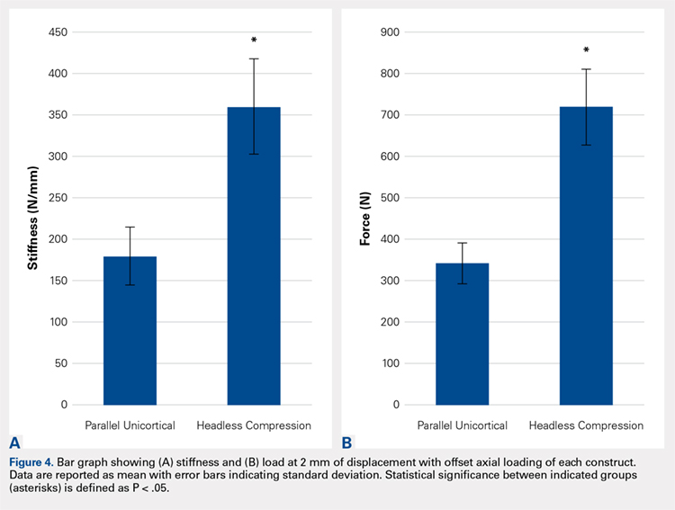
With offset axial testing to simulate supination-adduction force along with video motion analysis, the mean stiffness (± standard deviation) measured 180 ± 48 N/mm for the parallel unicortical screw fixation construct and 360 ± 131 N/mm for the headless compression screw fixation construct (Figure 4A). The headless compression screw fixation construct was over 2 times stiffer than the parallel unicortical construct during initial displacement of the fracture, indicating a statistically significant difference (P < .0001).
The mean force for 2 mm of fracture displacement, defined as clinical failure, reached 342 ± 83 N for the parallel unicortical screw fixation construct and 719 ± 91 N for the headless compression screw fixation construct (Figure 4B). The headless compression screw fixation construct resisted displacement significantly more (P = .0001) than the parallel unicortical screw construct, presenting a 100% increase.
Upon cycling of the servohydraulic testing machine back to 0-mm displacement, the parallel unicortical construct demonstrated no elastic recoil, remaining displaced at 4 mm, whereas the headless compression screw construct rebounded to almost 0-mm displacement, which is well below the clinical definition of fixation failure of 2 mm (Figure 5).
Continue to: Discussion...
DISCUSSION
When subjected to offset axial load, we observed that the headless compression screw construct exhibited significantly increased stiffness and load to 2 mm of displacement compared with a parallel unicortical screw construct. The headless compression screw also demonstrated elastic recoil to almost 0 mm of displacement, which is well below the 2-mm displacement.
We made reproducible fractures and fixation methods in synthetic distal tibiae, which feature less variability in size and quality than the cadaveric bone. Offset axial loading, rather than direct axial loading previously described by Amanatullah and colleagues,18 is the most physiologically relevant mode of force application to simulate the loading of the tauls onto the medial malleolus in the supination-adduction mechanism of injury.
The limitations of this study include the use of synthetic rather than cadaveric bone. Fourth-generation sawbones have been validated as possessing similar biomechanical properties as real bone.7,19 These results may also be inapplicable to osteoporotic bone, which would be significantly less dense than sawbones. This study is also an artificial situation designed to only test construct stiffness and load to clinical failure in a single mode of stress, offset axial loading and neglects other possible modes of force. This testing setup also disregards the structures surrounding the medial malleolus and tibia, including the talus, fibula, or soft tissue attachments, including the deltoid ligament and flexor retinaculum. These results are only relevant immediately after fixation and before bone healing occurs. We also tested the load to clinical failure rather than cyclic loading. Our testing more closely modeled a single traumatic force rather than the considerably smaller stresses that would be repeatedly exerted on the construct over several weeks after fixation in a clinical situation. This research is also not a clinical outcome study, rather, it suggests that headless compression screws are a viable, stronger, and possibly superior method for the initial fixation of vertical medial malleolar fractures.
As the load is offset axial, the larger thread purchase of the headless compression screws may lead to increased pullout strength, possibly increasing headless compression screw construct stiffness. Also, the variable diameter of headless compression screw, which reaches up to 4.7 mm, would increase the stiffness of the construct compared with the diameter of the cancellous screws. The elasticity of the headless compression construct may be because screws are made of titanium rather than stainless steel. Such property and given that the screws are cannulated rather than solid may also play a role, although several studies have shown variable results for cannulated vs solid screws of the same diameter.20,21 The elastic section modulus of both screws would have to be calculated to determine their exact effect on fixation.
CONCLUSION
The headless compression screw construct was found to be stiffer and features a higher load to clinical failure than a parallel unicortical cancellous screw construct for fixation of vertical medial malleolus fractures. Although significantly increased cost occurs with this construct, the headless design may decrease soft tissue irritation, and the elastic recoil of the construct after displacement may decrease clinical failure rates of this fixation method. This condition would eliminate the need for revision surgeries and thus be a cost effective alternative overall.
This paper will be judged for the Resident Writer’s Award.
- Fowler JR, Ilyas AM. Headless compression screw fixation of scaphoid fractures. Hand Clin. 2010;26(3):351-361, vi. doi:10.1016/j.hcl.2010.04.005.
- Karakasli A, Hapa O, Erduran M, Dincer C, Cecen B, Havitcioglu H. Mechanical comparison of headless screw fixation and locking plate fixation for talar neck fractures. J Foot Ankle Surg. 2015;54(5):905-909. doi:10.1053/j.jfas.2015.04.002.
- Elkowitz SJ, Polatsch DB, Egol KA, Kummer FJ, Koval KJ. Capitellum fractures: a biomechanical evaluation of three fixation methods. J Orthop Trauma. 2002;16(7):503-506. doi:10.1097/00005131-200208000-00009.
- Zhang H, Min L, Wang GL, et al. Primary open reduction and internal fixation with headless compression screws in the treatment of Chinese patients with acute Lisfranc joint injuries. J Trauma Acute Care Surg. 2012;72(5):1380-1385. doi:10.1097/TA.0b013e318246eabc.
- Lucas KJ, Morris RP, Buford WL Jr, Panchbhavi VK. Biomechanical comparison of first metatarsophalangeal joint arthrodeses using triple-threaded headless screws versus partially threaded lag screws. Foot Ankle Surg. 2014;20(2):144-148. doi:10.1016/j.fas.2014.02.009.
- Iwamoto T, Matsumura N, Sato K, Momohara S, Toyama Y, Nakamura T. An obliquely placed headless compression screw for distal interphalangeal joint arthrodesis. J Hand Surg. 2013;38(12):2360-2364. doi:10.1016/j.jhsa.2013.09.026.
- Odutola AA, Sheridan BD, Kelly AJ. Headless compression screw fixation prevents symptomatic metalwork in arthroscopic ankle arthrodesis. Foot Ankle Surg. 2012;18(2):111-113. doi:10.1016/j.fas.2011.03.013.
- Capelle JH, Couch CG, Wells KM, et al. Fixation strength of anteriorly inserted headless screws for talar neck fractures. Foot Ankle Int. 2013;34(7):1012-1016. doi:10.1177/1071100713479586.
- Wheeler DL, McLoughlin SW. Biomechanical assessment of compression screws. Clin Orthop Relat Res. 1998;350(350):237-245. doi:10.1097/00003086-199805000-00032.
- Rockwood CA, Green DP, Bucholz RW. Rockwood and Green's Fractures in Adults. 7th ed. Philadelphia, PA: Wolters Kluwer Health/Lippincott Williams & Wilkins; 2010.
- Simanski CJ, Maegele MG, Lefering R, et al. Functional treatment and early weightbearing after an ankle fracture: a prospective study. J Orthop Trauma. 2006;20(2):108-114. doi:10.1097/01.bot.0000197701.96954.8c.
- Reimer H, Kreibich M, Oettinger W. Extended uses for the Herbert/Whipple screw: six case reports out of 35 illustrating technique. J Orthop Trauma. 1996;10(1):7-14. doi:10.1097/00005131-199601000-00002.
- Barnes H, Cannada LK, Watson JT. A clinical evaluation of alternative fixation techniques for medial malleolus fractures. Injury. 2014;45(9):1365-1367. doi:10.1016/j.injury.2014.05.031.
- Dumigan RM, Bronson DG, Early JS. Analysis of fixation methods for vertical shear fractures of the medial malleolus. J Orthop Trauma. 2006;20(10):687-691. doi:10.1097/01.bot.0000247075.17548.3a.
- Toolan BC, Koval KJ, Kummer FJ, Sanders R, Zuckerman JD. Vertical shear fractures of the medial malleolus: a biomechanical study of five internal fixation techniques. Foot Ankle Int. 1994;15(9):483-489. doi:10.1177/107110079401500905.
- Ramsey PL, Hamilton W. Changes in tibiotalar area of contact caused by lateral talar shift. J Bone Joint Surg Am. 1976;58(3):356-357. doi:10.2106/00004623-197658030-00010.
- Thordarson DB, Motamed S, Hedman T, Ebramzadeh E, Bakshian S. The effect of fibular malreduction on contact pressures in an ankle fracture malunion model. J Bone Joint Surg Am. 1997;79(12):1809-1815. doi:10.2106/00004623-199712000-00006.
- Amanatullah DF, Khan SN, Curtiss S, Wolinsky PR. Effect of divergent screw fixation in vertical medial malleolus fractures. J Trauma Acute Care Surg. 2012;72(3):751-754. doi:10.1097/TA.0b013e31823b8b9f.
- Heiner AD. Structural properties of fourth-generation composite femurs and tibias. J Biomech. 2008;41(15):3282-3284. doi:10.1016/j.jbiomech.2008.08.013.
- Brown GA, McCarthy T, Bourgeault CA, Callahan DJ. Mechanical performance of standard and cannulated 4.0-mm cancellous bone screws. J Orthop Res. 2000;18(2):307-312. doi:10.1002/jor.1100180220.
- Merk BR, Stern SH, Cordes S, Lautenschlager EP. A fatigue life analysis of small fragment screws. J Orthop Trauma. 2001;15(7):494-499. doi:10.1097/00005131-200109000-00006.
ABSTRACT
This study is the first biomechanical research of headless compression screws for fixation of vertical shear fractures of the medial malleolus, a promising alternative that potentially offers several advantages for fixation.
Vertical shear fractures were simulated by osteotomies in 20 synthetic distal tibiae. Models were randomly assigned to fixation with either 2 parallel cancellous screws or 2 parallel Acutrak 2 headless compression screws (Acumed). Specimens were subjected to offset axial loading to simulate supination-adduction loading and tracked using high-resolution video.
The headless compression screw construct was significantly stiffer (P < .0001) (360 ± 131 N/mm) than the partially threaded cancellous screws (180 ± 48 N/mm) and demonstrated a significantly increased (P < .0001) mean load to clinical failure (719 ± 91 N vs 343 ± 83 N). When specimens were displaced to 6 mm and allowed to relax, the headless compression screw constructs demonstrated an elastic recoil and were reduced to the pretesting fragment alignment, whereas the parallel cancellous screw constructs remained displaced.
Along with the headless design that may decrease soft tissue irritation, the increased stiffness and elastic recoil of the headless compression screw construct offers improved fixation of medial malleolus vertical shear fractures over the traditional methods.
Continue to: Headless compressions screws...
Headless compressions screws are cannulated tapered titanium screws with variable thread pitch angle, allowing a fully threaded screw to apply compression along its entire length. These screws have been most commonly used for scaphoid fractures1 but have also been studied in fractures of small bones, such as capitellum, midfoot, and talar neck,2-4 and arthrodesis in the foot, ankle, and hand.5-7 Headless compression screws have been found to produce equivalent fragment compression to partially threaded cancellous screws while allowing less fragment displacement.8,9 The lack of a head may decrease soft tissue irritation compared with the partially threaded cancellous screws. Finally, headless compression screws are independent of cortical integrity, as the entire length of the screw features a wide thread diameter to capture cancellous bone in the proximal fragment, unlike partially threaded cancellous screws, which only possess a thread purchase in the distal fragment and depend on an intact cortex.
Vertical shear fractures of the medial malleolus occur through the supination-adduction of the talus exerted onto the articular surface of the medial malleolus.10 Optimal fixation of these fractures must be sufficient to maintain stable anatomic reduction of the ankle joint articular surface, allowing early range of motion, maintaining congruency of the ankle joint, and decreasing the risk of future post-traumatic arthritis to maximize functional outcome.11
A wide variety of techniques are available for fixation of these fractures, including various configurations of cortical screws, cancellous screws, tension bands, and antiglide plates. Clinically, 2 parallel 4.0-mm partially threaded cancellous screws are most often used. Limited evidence indicates that headless compression screws may be a viable option for fixation of medial malleolus fractures. One case reports the use of a headless compression screw for a horizontal medial malleolar fracture,12 and a small retrospective case series that used headless compression screws for all medial malleolar fractures showed satisfactory outcomes, a high union rate, and low patient-reported pain.13
We evaluate the stiffness, force to 2-mm displacement of the joint surface, and elastic properties of these 2 different constructs in vertical medial malleolar fractures in synthetic distal tibiae. We hypothesize that the parallel headless compression screw fixation will be stiffer and require more force to 2-mm displacement than parallel unicortical cancellous screw fixation.
MATERIALS AND METHODS
Identical vertical osteotomies (17.5 mm) were made from the medial border of the medial malleolus using a custom jig in 20 left 4th-generation composite synthetic distal tibiae (Sawbones, Pacific Research Labs; Model No. 3401) to simulate an Orthopaedic Trauma Association type 44-A2.3 fracture. The tibiae were then cut 18 cm from the tibial plafond and randomized to 2 fixation groups (n = 10 specimens for each group): parallel unicortical screw fixation or parallel unicortical headless compression screw fixation (Figures 1A-1D). Custom polymethylmethacrylate jigs were used to reproducibly drill identical holes with a 3.2-mm drill for the parallel unicortical screw construct and the drill bits provided by the Acutrak 2 Headless Compression Screw System (Acumed). The parallel unicortical screw construct consisted of 2 parallel 4.0-mm-diameter, 40-mm partially threaded cancellous screws (Depuy Synthes), and the headless compression fixation construct consisted of 2 parallel 4.7-mm-diameter, 45-mm titanium Acutrak 2 screws parallel to each other in the transverse plane. The Acutrak screws were placed per manufacturer instructions by first drilling with the Acutrak 2-4.7 Long Drill bit (Acumed), followed by the Acutrak 2-4.7 Profile Drill bit for the near cortex.
Continue to: Specimens...
Specimens were fixed to the base of a servohydraulic testing machine (Model 809, MTS Systems Corporation) with an axial-torsional load transducer (Model No. 662.20-01; Axial capacity of 250 kg, torsional capacity 2.88 kg-m; MTS Systems Corporation). The specimens were set in a vice tilted at 17° in the coronal plane to allow the MTS crosshead to apply an offset axial load simulating supination-adduction loading, which has been described previously (Figure 2).14,15 Load was applied to the inferolateral articular surface of the medial malleolus at 1 mm/s to a crosshead displacement of 6 mm and then cycled back to 0 mm. Load and axial displacement were measured at 60 Hz. The markers on the distal tibia and medial malleolus fracture fragment were tracked using high-resolution video (Fastcam PCI, Photron USA Inc). The motion of the video markers was determined using digitization and motion analysis software (Motus 9, Vicon).
Stiffness was calculated as the slope of the linear portion of the load-displacement curve over a range of 0.5 to 2.0 mm (Figure 3) and reported as mean (standard deviation). The force at 2 mm of fragment displacement was defined as a clinical failure.16,17 Student’s t test was used to determine the difference in construct stiffness and force for 2 mm displacement of the 2 groups. Significance was defined as P < .05. Institutional Review Board approval was not required for this study.
RESULTS
With offset axial testing to simulate supination-adduction force along with video motion analysis, the mean stiffness (± standard deviation) measured 180 ± 48 N/mm for the parallel unicortical screw fixation construct and 360 ± 131 N/mm for the headless compression screw fixation construct (Figure 4A). The headless compression screw fixation construct was over 2 times stiffer than the parallel unicortical construct during initial displacement of the fracture, indicating a statistically significant difference (P < .0001).
The mean force for 2 mm of fracture displacement, defined as clinical failure, reached 342 ± 83 N for the parallel unicortical screw fixation construct and 719 ± 91 N for the headless compression screw fixation construct (Figure 4B). The headless compression screw fixation construct resisted displacement significantly more (P = .0001) than the parallel unicortical screw construct, presenting a 100% increase.
Upon cycling of the servohydraulic testing machine back to 0-mm displacement, the parallel unicortical construct demonstrated no elastic recoil, remaining displaced at 4 mm, whereas the headless compression screw construct rebounded to almost 0-mm displacement, which is well below the clinical definition of fixation failure of 2 mm (Figure 5).
Continue to: Discussion...
DISCUSSION
When subjected to offset axial load, we observed that the headless compression screw construct exhibited significantly increased stiffness and load to 2 mm of displacement compared with a parallel unicortical screw construct. The headless compression screw also demonstrated elastic recoil to almost 0 mm of displacement, which is well below the 2-mm displacement.
We made reproducible fractures and fixation methods in synthetic distal tibiae, which feature less variability in size and quality than the cadaveric bone. Offset axial loading, rather than direct axial loading previously described by Amanatullah and colleagues,18 is the most physiologically relevant mode of force application to simulate the loading of the tauls onto the medial malleolus in the supination-adduction mechanism of injury.
The limitations of this study include the use of synthetic rather than cadaveric bone. Fourth-generation sawbones have been validated as possessing similar biomechanical properties as real bone.7,19 These results may also be inapplicable to osteoporotic bone, which would be significantly less dense than sawbones. This study is also an artificial situation designed to only test construct stiffness and load to clinical failure in a single mode of stress, offset axial loading and neglects other possible modes of force. This testing setup also disregards the structures surrounding the medial malleolus and tibia, including the talus, fibula, or soft tissue attachments, including the deltoid ligament and flexor retinaculum. These results are only relevant immediately after fixation and before bone healing occurs. We also tested the load to clinical failure rather than cyclic loading. Our testing more closely modeled a single traumatic force rather than the considerably smaller stresses that would be repeatedly exerted on the construct over several weeks after fixation in a clinical situation. This research is also not a clinical outcome study, rather, it suggests that headless compression screws are a viable, stronger, and possibly superior method for the initial fixation of vertical medial malleolar fractures.
As the load is offset axial, the larger thread purchase of the headless compression screws may lead to increased pullout strength, possibly increasing headless compression screw construct stiffness. Also, the variable diameter of headless compression screw, which reaches up to 4.7 mm, would increase the stiffness of the construct compared with the diameter of the cancellous screws. The elasticity of the headless compression construct may be because screws are made of titanium rather than stainless steel. Such property and given that the screws are cannulated rather than solid may also play a role, although several studies have shown variable results for cannulated vs solid screws of the same diameter.20,21 The elastic section modulus of both screws would have to be calculated to determine their exact effect on fixation.
CONCLUSION
The headless compression screw construct was found to be stiffer and features a higher load to clinical failure than a parallel unicortical cancellous screw construct for fixation of vertical medial malleolus fractures. Although significantly increased cost occurs with this construct, the headless design may decrease soft tissue irritation, and the elastic recoil of the construct after displacement may decrease clinical failure rates of this fixation method. This condition would eliminate the need for revision surgeries and thus be a cost effective alternative overall.
This paper will be judged for the Resident Writer’s Award.
- Fowler JR, Ilyas AM. Headless compression screw fixation of scaphoid fractures. Hand Clin. 2010;26(3):351-361, vi. doi:10.1016/j.hcl.2010.04.005.
- Karakasli A, Hapa O, Erduran M, Dincer C, Cecen B, Havitcioglu H. Mechanical comparison of headless screw fixation and locking plate fixation for talar neck fractures. J Foot Ankle Surg. 2015;54(5):905-909. doi:10.1053/j.jfas.2015.04.002.
- Elkowitz SJ, Polatsch DB, Egol KA, Kummer FJ, Koval KJ. Capitellum fractures: a biomechanical evaluation of three fixation methods. J Orthop Trauma. 2002;16(7):503-506. doi:10.1097/00005131-200208000-00009.
- Zhang H, Min L, Wang GL, et al. Primary open reduction and internal fixation with headless compression screws in the treatment of Chinese patients with acute Lisfranc joint injuries. J Trauma Acute Care Surg. 2012;72(5):1380-1385. doi:10.1097/TA.0b013e318246eabc.
- Lucas KJ, Morris RP, Buford WL Jr, Panchbhavi VK. Biomechanical comparison of first metatarsophalangeal joint arthrodeses using triple-threaded headless screws versus partially threaded lag screws. Foot Ankle Surg. 2014;20(2):144-148. doi:10.1016/j.fas.2014.02.009.
- Iwamoto T, Matsumura N, Sato K, Momohara S, Toyama Y, Nakamura T. An obliquely placed headless compression screw for distal interphalangeal joint arthrodesis. J Hand Surg. 2013;38(12):2360-2364. doi:10.1016/j.jhsa.2013.09.026.
- Odutola AA, Sheridan BD, Kelly AJ. Headless compression screw fixation prevents symptomatic metalwork in arthroscopic ankle arthrodesis. Foot Ankle Surg. 2012;18(2):111-113. doi:10.1016/j.fas.2011.03.013.
- Capelle JH, Couch CG, Wells KM, et al. Fixation strength of anteriorly inserted headless screws for talar neck fractures. Foot Ankle Int. 2013;34(7):1012-1016. doi:10.1177/1071100713479586.
- Wheeler DL, McLoughlin SW. Biomechanical assessment of compression screws. Clin Orthop Relat Res. 1998;350(350):237-245. doi:10.1097/00003086-199805000-00032.
- Rockwood CA, Green DP, Bucholz RW. Rockwood and Green's Fractures in Adults. 7th ed. Philadelphia, PA: Wolters Kluwer Health/Lippincott Williams & Wilkins; 2010.
- Simanski CJ, Maegele MG, Lefering R, et al. Functional treatment and early weightbearing after an ankle fracture: a prospective study. J Orthop Trauma. 2006;20(2):108-114. doi:10.1097/01.bot.0000197701.96954.8c.
- Reimer H, Kreibich M, Oettinger W. Extended uses for the Herbert/Whipple screw: six case reports out of 35 illustrating technique. J Orthop Trauma. 1996;10(1):7-14. doi:10.1097/00005131-199601000-00002.
- Barnes H, Cannada LK, Watson JT. A clinical evaluation of alternative fixation techniques for medial malleolus fractures. Injury. 2014;45(9):1365-1367. doi:10.1016/j.injury.2014.05.031.
- Dumigan RM, Bronson DG, Early JS. Analysis of fixation methods for vertical shear fractures of the medial malleolus. J Orthop Trauma. 2006;20(10):687-691. doi:10.1097/01.bot.0000247075.17548.3a.
- Toolan BC, Koval KJ, Kummer FJ, Sanders R, Zuckerman JD. Vertical shear fractures of the medial malleolus: a biomechanical study of five internal fixation techniques. Foot Ankle Int. 1994;15(9):483-489. doi:10.1177/107110079401500905.
- Ramsey PL, Hamilton W. Changes in tibiotalar area of contact caused by lateral talar shift. J Bone Joint Surg Am. 1976;58(3):356-357. doi:10.2106/00004623-197658030-00010.
- Thordarson DB, Motamed S, Hedman T, Ebramzadeh E, Bakshian S. The effect of fibular malreduction on contact pressures in an ankle fracture malunion model. J Bone Joint Surg Am. 1997;79(12):1809-1815. doi:10.2106/00004623-199712000-00006.
- Amanatullah DF, Khan SN, Curtiss S, Wolinsky PR. Effect of divergent screw fixation in vertical medial malleolus fractures. J Trauma Acute Care Surg. 2012;72(3):751-754. doi:10.1097/TA.0b013e31823b8b9f.
- Heiner AD. Structural properties of fourth-generation composite femurs and tibias. J Biomech. 2008;41(15):3282-3284. doi:10.1016/j.jbiomech.2008.08.013.
- Brown GA, McCarthy T, Bourgeault CA, Callahan DJ. Mechanical performance of standard and cannulated 4.0-mm cancellous bone screws. J Orthop Res. 2000;18(2):307-312. doi:10.1002/jor.1100180220.
- Merk BR, Stern SH, Cordes S, Lautenschlager EP. A fatigue life analysis of small fragment screws. J Orthop Trauma. 2001;15(7):494-499. doi:10.1097/00005131-200109000-00006.
TAKE-HOME POINTS
- Optimal fixation of vertical sheer ankle fractures is unknown.
- Headless compression screws are stiffer than cancellous screws in offset axial load.
- Headless compression screws have a higher load to failure than cancellous screws.
- Headless compression screws may offer a soft tissue friendly fixation of method for vertical sheer ankle fractures.
- These findings may not apply when subject to cyclic loads or in osteoporotic bone.
Having prescription drug coverage is associated with improved myeloma outcomes
Medicare beneficiaries with myeloma who have prescription drug coverage have shown both decreased used of classic cytotoxic chemotherapy and better survival, according to new research.

The findings suggested that prescription drug coverage brings better access to all existing treatment options.
“In this analysis of Medicare beneficiaries with myeloma, the receipt of therapy and survival differed according to prescription drug coverage status,” Adam Olszewski, MD, of the Lifespan Cancer Institute at Rhode Island Hospital in Providence, R.I., and his colleagues noted in the study. “Patients with PDP [prescription drug plan coverage through Medicare Part D] or OCC [other credible prescription drug coverage] more often received active myeloma care, compared to those without coverage,” they wrote in Journal of Clinical Oncology.
The researchers looked at 9,755 patients diagnosed with myeloma during 2006-2011 and examined what was used to treat the myeloma as a first line treatment. The cohort included 1,460 patients with no prescription drug coverage, 3,283 with PDP coverage, 3,607 with OCC, and 1,405 dual eligibility for Medicare and Medicaid coverage.
The study found that, compared with beneficiaries with no coverage, Medicare beneficiaries with PDP coverage “were 14% less likely to be treated with parenteral chemotherapy and 38% less likely to receive classic cytotoxic agents.” Additionally, among the cohort of beneficiaries that were without drug coverage prior to the diagnosis of myeloma, 41% actively obtained coverage, but even then, their survival was “significantly worse, compared with the beneficiaries who had coverage at diagnosis.”
Beneficiaries classified as having other credible coverage were 3% more likely to receive active myeloma care than were those without coverage, but the use of parenteral regimens did not differ between those groups.
Researchers noted that overall survival was 10% higher at 1 year and 6% higher at 3 years for beneficiaries with PDP coverage or OCC than it was for those without coverage, but they added that the analysis required cautious interpretation “as it is confounded by multiple baseline factors and mediated by the quality of cancer treatment. ... We could not discern whether worse survival in the group without coverage was a result of not receiving therapy at all, an inability to access IMiDs [immunomodulatory drugs], or poor control of other medical issues.”
However, a comparison with the control group “strongly suggest[s] that patients with myeloma without prescription drug coverage may not have received the most effective first-line therapy,” Dr. Olszewski and his colleagues added. “Survival for PDP and OCC groups remained identical, which supports the notion that having any prescription drug coverage contributed to optimal treatment and outcomes.”
The study was limited by the fact that unobserved clinical differences between beneficiaries with or without prescription drug coverage could have accounted for differences in mortality and that the comparison of treatments was restricted to parenteral regimens because IMiDs were observed to have been administered only for PDP enrollees.
Dr. Olszewski and study coauthor Amy Davidoff, PhD, of Yale University, New Haven, Conn., disclosed acting in consulting or advisory roles and receiving research funding from several pharmaceutical companies that develop cancer treatments.
SOURCE: Olszewski A et al. J Clin Oncol. 2018 Aug 16. doi: 10.1200/JCO.2018.77.8894.
Medicare beneficiaries with myeloma who have prescription drug coverage have shown both decreased used of classic cytotoxic chemotherapy and better survival, according to new research.
The findings suggested that prescription drug coverage brings better access to all existing treatment options.
“In this analysis of Medicare beneficiaries with myeloma, the receipt of therapy and survival differed according to prescription drug coverage status,” Adam Olszewski, MD, of the Lifespan Cancer Institute at Rhode Island Hospital in Providence, R.I., and his colleagues noted in the study. “Patients with PDP [prescription drug plan coverage through Medicare Part D] or OCC [other credible prescription drug coverage] more often received active myeloma care, compared to those without coverage,” they wrote in Journal of Clinical Oncology.
The researchers looked at 9,755 patients diagnosed with myeloma during 2006-2011 and examined what was used to treat the myeloma as a first line treatment. The cohort included 1,460 patients with no prescription drug coverage, 3,283 with PDP coverage, 3,607 with OCC, and 1,405 dual eligibility for Medicare and Medicaid coverage.
The study found that, compared with beneficiaries with no coverage, Medicare beneficiaries with PDP coverage “were 14% less likely to be treated with parenteral chemotherapy and 38% less likely to receive classic cytotoxic agents.” Additionally, among the cohort of beneficiaries that were without drug coverage prior to the diagnosis of myeloma, 41% actively obtained coverage, but even then, their survival was “significantly worse, compared with the beneficiaries who had coverage at diagnosis.”
Beneficiaries classified as having other credible coverage were 3% more likely to receive active myeloma care than were those without coverage, but the use of parenteral regimens did not differ between those groups.
Researchers noted that overall survival was 10% higher at 1 year and 6% higher at 3 years for beneficiaries with PDP coverage or OCC than it was for those without coverage, but they added that the analysis required cautious interpretation “as it is confounded by multiple baseline factors and mediated by the quality of cancer treatment. ... We could not discern whether worse survival in the group without coverage was a result of not receiving therapy at all, an inability to access IMiDs [immunomodulatory drugs], or poor control of other medical issues.”
However, a comparison with the control group “strongly suggest[s] that patients with myeloma without prescription drug coverage may not have received the most effective first-line therapy,” Dr. Olszewski and his colleagues added. “Survival for PDP and OCC groups remained identical, which supports the notion that having any prescription drug coverage contributed to optimal treatment and outcomes.”
The study was limited by the fact that unobserved clinical differences between beneficiaries with or without prescription drug coverage could have accounted for differences in mortality and that the comparison of treatments was restricted to parenteral regimens because IMiDs were observed to have been administered only for PDP enrollees.
Dr. Olszewski and study coauthor Amy Davidoff, PhD, of Yale University, New Haven, Conn., disclosed acting in consulting or advisory roles and receiving research funding from several pharmaceutical companies that develop cancer treatments.
SOURCE: Olszewski A et al. J Clin Oncol. 2018 Aug 16. doi: 10.1200/JCO.2018.77.8894.
FROM THE JOURNAL OF CLINICAL ONCOLOGY
Key clinical point: Prescription drug coverage is related to better outcomes for Medicare patients with myeloma.
Major finding: Compared with patients without coverage, patients with prescription drug plan coverage through Medicare Part D were 14% less likely to receive parenteral chemotherapy and 38% less likely to receive classic cytotoxic agents.
Study details: Observational study using SEER-Medicare data for 9,755 beneficiaries diagnosed with myeloma during 2006-2011.
Disclosures: The study was supported by scholar awards from the American Cancer Society and the American Society of Hematology and by a grant from the National Institute of General Medical Sciences. Report authors Dr. Olszewski and one coauthor disclosed receiving research funding and other financial compensation from several pharmaceutical companies that develop cancer treatments.
Source: Olszewski A et al. J Clin Oncol. 2018 Aug 16. doi: 10.1200/JCO.2018.77.8894
Innovations Lead to More Targeted Prostate Cancer Treatments (FULL)
The main treatment for prostate cancer—the third leading cause of cancer death in American men—often is “watchful waiting.” But what happens before, during, and after that waiting period has changed tremendously in recent years. Innovative and improved methods and drugs allow for a more precise diagnosis, better risk stratification, targeted treatment options, and longer survival.
Innovations in diagnosis include a revised histologic grading system, which was incorporated into the 2016 World Health Organization classification of tumors. The new grading system ranks prostate cancer on a 1-to-5 scale, making it more discriminating, as validated in a study of more than 25,000 men.
The use of new prognostic biomarkers has advanced risk stratification. According to a recent review, biopsy guided by ultrasound misses between 21% and 28% of prostate cancers and undergrades between 14% and 17%.1 But new serum-, tissue-, and image-based biomarkers may help identify potential false negatives. The prostate cancer antigen 3 test, for example, has an 88% negative predictive value for subsequent biopsy. Molecular biomarkers also can predict clinical progression, risk of adverse pathology, and metastatic risk.
Fortunately, biopsy guided by ultrasound is getting more precise. Advances in magnetic resonance imaging (MRI) now allow for “targeted biopsies.” The enhanced MRI has 89% sensitivity and 73% specificity for identifying prostate cancer. According to one study of 1,003 men, targeted prostate biopsy using MRI-ultrasound fusion identified 30% more cases of Gleason score ≥ 4 + 3 than did systematic prostate biopsy.1 Updates in positron emission tomography are garnering interest for improved staging because this technology allows for better detection of local recurrence, regional lymph node metastases, and distant metastases.
Once a prostate cancer diagnosis has been confirmed, the decision of what to do next may be watchful waiting (treating symptoms palliatively), but recent research suggests that active surveillance that includes regular prostate-specific antigen testing, physical examinations, and prostate biopsies may be a better choice, particularly for men with less aggressive cancer. One study of 1,298 men with mostly very low-risk disease followed for up to 60 months found metastasis in only 5; only 2 died. The Prostate Testing for Cancer and Treatment (ProtecT) trial found that the number of deaths in the active monitoring group did not differ significantly from those in the surgery or radiation groups.
What should be the contemporary standard of care? Androgen deprivation therapy (ADT) is still the go-to treatment for men with metastatic prostate cancer. Although ADT has been associated with toxicity, a meta-analysis found continuous ADT was better than intermittent in terms of disease progression and survival.1
Other research has focused on which types of prostate cancer respond best to specific therapies. Molecular subtyping (already available in bladder and breast cancer) is gaining popularity. Prostate cancer was thought to derive from glandular luminal cells, but recent evidence supports the idea that basal cells play a role as well. Researchers who analyzed nearly 4,000 samples suggest that luminal B tumors respond better to postoperative ADT than do nonluminal B cancers. These findings suggest that “personalized” ADT treatment may be possible.2
Several drugs have been shown to improve survival: Among them, docetaxel, abiraterone acetate, enzalutamide, and cabazitaxel. In the STAMPEDE trial, men with locally advanced or metastatic prostate cancer who received ADT plus abiraterone and prednisolone had significantly higher rates of overall and failure-free survival.3
Docetaxel, which can extend survival by 10 to 13 months compared with standard ADT, is taking on a bigger role for its ability to delay progression and recurrence while being well tolerated. Options for men whose cancer does not respond to ADT include abiraterone and enzalutamide. Both act on the androgen axis to slow progression and improve survival.
More than 30% of patients treated with radical prostatectomy will have recurrent cancer as will 50% of those treated with salvage radiation therapy. Bicalutamide has shown extremely promising action against recurrent cancer. In one study, the cumulative incidence of metastatic prostate cancer at 12 years was 14.5% in the bicalutamide group, compared with 23.0% in the placebo group.4
But while that study was going on, it was superseded by injectable gonadotropin-releasing hormone agonists as first-choice hormonal therapy with radiation. However, the researchers say that does not
Multimodal therapy and precision medicine are becoming bywords in prostate cancer treatment. Drugs on the horizon likely will be tailored to tumor molecular biology, with genetic information used to specifically guide diagnosis and treatment. Prostate cancer may still be a slow killer, but immunotherapies (like sipuleucel-T, the first FDA-approved cancer vaccine), hormonal therapies, and bone-targeting agents enable men with prostate cancer to not only live longer but also with a better quality of life.
Click here to read the digital edition.
1. Litwin MS, Tan HJ. The diagnosis and treatment of prostate cancer: a review. JAMA. 2017;317(24):2532-2542.
2. Zhao SG, Chang SL, Erho N, et al. Associations of luminal and basal subtyping of prostate cancer with prognosis and response to androgen deprivation therapy. JAMA Oncol. 2017. [Epub ahead of print.]
3. James ND, de Bono JS, Spears MR, et al; for the STAMPEDE Investigators. Abiraterone for prostate cancer not previously treated with hormone therapy. N Engl J Med. 2017. [Epub ahead of print.]
4. Shipley WU, Seiferheld W, Lukka HR, et al; NRG Oncology RTOG. Radiation with or without antiandrogen therapy in recurrent prostate cancer. N Engl J Med. 2017;376(5):417-428.
The main treatment for prostate cancer—the third leading cause of cancer death in American men—often is “watchful waiting.” But what happens before, during, and after that waiting period has changed tremendously in recent years. Innovative and improved methods and drugs allow for a more precise diagnosis, better risk stratification, targeted treatment options, and longer survival.
Innovations in diagnosis include a revised histologic grading system, which was incorporated into the 2016 World Health Organization classification of tumors. The new grading system ranks prostate cancer on a 1-to-5 scale, making it more discriminating, as validated in a study of more than 25,000 men.
The use of new prognostic biomarkers has advanced risk stratification. According to a recent review, biopsy guided by ultrasound misses between 21% and 28% of prostate cancers and undergrades between 14% and 17%.1 But new serum-, tissue-, and image-based biomarkers may help identify potential false negatives. The prostate cancer antigen 3 test, for example, has an 88% negative predictive value for subsequent biopsy. Molecular biomarkers also can predict clinical progression, risk of adverse pathology, and metastatic risk.
Fortunately, biopsy guided by ultrasound is getting more precise. Advances in magnetic resonance imaging (MRI) now allow for “targeted biopsies.” The enhanced MRI has 89% sensitivity and 73% specificity for identifying prostate cancer. According to one study of 1,003 men, targeted prostate biopsy using MRI-ultrasound fusion identified 30% more cases of Gleason score ≥ 4 + 3 than did systematic prostate biopsy.1 Updates in positron emission tomography are garnering interest for improved staging because this technology allows for better detection of local recurrence, regional lymph node metastases, and distant metastases.
Once a prostate cancer diagnosis has been confirmed, the decision of what to do next may be watchful waiting (treating symptoms palliatively), but recent research suggests that active surveillance that includes regular prostate-specific antigen testing, physical examinations, and prostate biopsies may be a better choice, particularly for men with less aggressive cancer. One study of 1,298 men with mostly very low-risk disease followed for up to 60 months found metastasis in only 5; only 2 died. The Prostate Testing for Cancer and Treatment (ProtecT) trial found that the number of deaths in the active monitoring group did not differ significantly from those in the surgery or radiation groups.
What should be the contemporary standard of care? Androgen deprivation therapy (ADT) is still the go-to treatment for men with metastatic prostate cancer. Although ADT has been associated with toxicity, a meta-analysis found continuous ADT was better than intermittent in terms of disease progression and survival.1
Other research has focused on which types of prostate cancer respond best to specific therapies. Molecular subtyping (already available in bladder and breast cancer) is gaining popularity. Prostate cancer was thought to derive from glandular luminal cells, but recent evidence supports the idea that basal cells play a role as well. Researchers who analyzed nearly 4,000 samples suggest that luminal B tumors respond better to postoperative ADT than do nonluminal B cancers. These findings suggest that “personalized” ADT treatment may be possible.2
Several drugs have been shown to improve survival: Among them, docetaxel, abiraterone acetate, enzalutamide, and cabazitaxel. In the STAMPEDE trial, men with locally advanced or metastatic prostate cancer who received ADT plus abiraterone and prednisolone had significantly higher rates of overall and failure-free survival.3
Docetaxel, which can extend survival by 10 to 13 months compared with standard ADT, is taking on a bigger role for its ability to delay progression and recurrence while being well tolerated. Options for men whose cancer does not respond to ADT include abiraterone and enzalutamide. Both act on the androgen axis to slow progression and improve survival.
More than 30% of patients treated with radical prostatectomy will have recurrent cancer as will 50% of those treated with salvage radiation therapy. Bicalutamide has shown extremely promising action against recurrent cancer. In one study, the cumulative incidence of metastatic prostate cancer at 12 years was 14.5% in the bicalutamide group, compared with 23.0% in the placebo group.4
But while that study was going on, it was superseded by injectable gonadotropin-releasing hormone agonists as first-choice hormonal therapy with radiation. However, the researchers say that does not
Multimodal therapy and precision medicine are becoming bywords in prostate cancer treatment. Drugs on the horizon likely will be tailored to tumor molecular biology, with genetic information used to specifically guide diagnosis and treatment. Prostate cancer may still be a slow killer, but immunotherapies (like sipuleucel-T, the first FDA-approved cancer vaccine), hormonal therapies, and bone-targeting agents enable men with prostate cancer to not only live longer but also with a better quality of life.
Click here to read the digital edition.
1. Litwin MS, Tan HJ. The diagnosis and treatment of prostate cancer: a review. JAMA. 2017;317(24):2532-2542.
2. Zhao SG, Chang SL, Erho N, et al. Associations of luminal and basal subtyping of prostate cancer with prognosis and response to androgen deprivation therapy. JAMA Oncol. 2017. [Epub ahead of print.]
3. James ND, de Bono JS, Spears MR, et al; for the STAMPEDE Investigators. Abiraterone for prostate cancer not previously treated with hormone therapy. N Engl J Med. 2017. [Epub ahead of print.]
4. Shipley WU, Seiferheld W, Lukka HR, et al; NRG Oncology RTOG. Radiation with or without antiandrogen therapy in recurrent prostate cancer. N Engl J Med. 2017;376(5):417-428.
Broad genomic testing of NSCLC in community oncology disappoints
results of a retrospective cohort study reported in JAMA suggest.
Investigators led by Carolyn J. Presley, MD, a thoracic and geriatric medical oncologist at the Ohio State University Comprehensive Cancer Center, Columbus, assessed outcomes among more than 5,500 patients with advanced nonsquamous NSCLC treated mainly in U.S. community practices. Overall, 15% had broad-based genomic testing (next-generation sequencing evaluating more than 30 cancer genes).
Main results showed that, among the patients having broad testing, less than 5% received a targeted treatment based on results that were not attainable with routine testing for common alterations in EGFR and ALK genes. Moreover, survival after broad testing was not better than that after routine testing.
“This study highlights how broad-based genomic sequencing has disseminated beyond traditional research settings ahead of a demonstrated association with better survival,” Dr. Presley and her coinvestigators write. They speculate that community uptake is being driven by the ease and cost of ordering a single comprehensive test, perceived benefit, attempts to conserve tissue, and hopes of improved survival if a targeted treatment is available.
“The lack of an association between broad-based genomic sequencing and survival is likely multifactorial,” the investigators maintain. “First, there were few genetic alterations identified with available targeted treatments. Second, even among those patients for whom targeted treatments were available, the treatments may not yield a substantial survival benefit or patients may not have had access to targeted agents due to financial barriers. Decision support for clinicians once they receive broad-based genomic sequencing results may also be needed.”
Study details
Dr. Presley and colleagues used the Flatiron Health Database to identify patients with advanced NSCLC who received care at 191 oncology practices across the United States during 2011-2016. The 5,688 patients studied had stage IIIB, stage IV, or unresectable nonsquamous NSCLC and received at least one line of treatment.
Overall, 15.4% received broad-based genomic sequencing of their tumor, while the rest received routine testing for EGFR and/or ALK alterations only, according to the results reported.
In the broadly tested group, merely 4.5% were given targeted treatment based on testing results. Another 9.8% received routine EGFR/ALK-targeted treatment, and 85.1% did not receive any targeted treatment.
The 12-month unadjusted mortality rate was 49.2% for patients undergoing broad testing, compared with 35.9% for patients undergoing routine testing.
In an instrumental variable analysis done to account for confounding, the 12-month predicted probability of death was 41.1% after broad testing and 44.4% after routine testing (P = .63).
Findings were similar in a propensity score–matched survival analysis (42.0% vs. 45.1%; hazard ratio, 0.92; P = .40), although there was some suggestion of a benefit of broad testing over routine testing in a Kaplan-Meier analysis among the entire unmatched cohort (HR, 0.69; P less than .001).
“Improved access to research clinical trials in the community setting may improve use of mutational data,” the investigators speculate. “Given the paucity of targeted agents, efforts to increase access to broad-based genomic sequencing should be paired with efforts to facilitate clinical trial enrollment.”
Dr. Presley disclosed that she receives grants from the Yale Lung SPORE Career Development Award, the Robert Wood Johnson/Veterans Affairs Clinical Scholars Program, and The Ohio State University K12 Training Grant for clinical faculty investigators. The study was funded by the Veterans Affairs Robert Wood Johnson Clinical Scholar Program and the Yale Lung SPORE Career Development Award.
SOURCE: Presley CJ et al. JAMA. 2018 Aug 7. doi: 10.1001/jama.2018.9824.
There still may be a role for broad-based genomic testing in patients with NSCLC treated in community oncology practices, according to editorialists Paul A. Bunn Jr., MD, and Dara L. Aisner, MD, PhD. They discussed several study limitations that leave the matter unsettled.
Importantly, the majority of patients in whom this testing identified a potentially treatable alteration did not receive the treatment. “This gap between finding and treating molecular alterations in the community-based clinical setting highlights the reality that obtaining more tumor genomic information must be complemented with clinician education and decision support to understand the importance of matched therapy, and demonstrates a strength of harnessing EMR data to identify potential gaps in practice,” they maintain.
The study did not assess important outcomes other than survival, such as progression-free survival and response rate, Dr. Bunn and Dr. Aisner further note. Previous research has shown that tyrosine kinase inhibitors, for example, improve some of these outcomes without altering survival.
Another limitation was that the study period predated regulatory approval of some relevant targeted therapies and came shortly on the heels of approval of a targeted therapy for ALK rearrangements. And additional therapies are in the pipeline.
“[T]he incremental value of a cutoff of 30 genes analyzed may place the bar too high to appreciate a survival advantage and the tissue, time, and cost savings due to next-generation sequencing were not considered,” the editorialists point out. The optimal number of genes is unclear and likely to change over time.
Finally, the reports oncologists receive from broad-based genomic sequencing may be long and complex, which may deter them from pursuing appropriate therapy, Dr. Bunn and Dr. Aisner propose.
“The study… provides important insights into how broad-based genomic sequencing is used in the community oncology setting, where the majority of patients with advanced NSCLC in the United States receive care,” they conclude. “However, the limitations of this investigation suggest that the authors’ conclusion that broad testing is not warranted should be tempered to ensure that patients receive the right therapy for the right alteration at the right time.”
Paul A. Bunn Jr., MD, is with the University of Colorado Cancer Center and department of medical oncology, University of Colorado, Denver and Dara L. Aisner, MD, PhD, is with the University of Colorado Cancer Center and department of pathology, University of Colorado, Aurora. These comments were excerpted from an accompanying editorial .
results of a retrospective cohort study reported in JAMA suggest.
Investigators led by Carolyn J. Presley, MD, a thoracic and geriatric medical oncologist at the Ohio State University Comprehensive Cancer Center, Columbus, assessed outcomes among more than 5,500 patients with advanced nonsquamous NSCLC treated mainly in U.S. community practices. Overall, 15% had broad-based genomic testing (next-generation sequencing evaluating more than 30 cancer genes).
Main results showed that, among the patients having broad testing, less than 5% received a targeted treatment based on results that were not attainable with routine testing for common alterations in EGFR and ALK genes. Moreover, survival after broad testing was not better than that after routine testing.
“This study highlights how broad-based genomic sequencing has disseminated beyond traditional research settings ahead of a demonstrated association with better survival,” Dr. Presley and her coinvestigators write. They speculate that community uptake is being driven by the ease and cost of ordering a single comprehensive test, perceived benefit, attempts to conserve tissue, and hopes of improved survival if a targeted treatment is available.
“The lack of an association between broad-based genomic sequencing and survival is likely multifactorial,” the investigators maintain. “First, there were few genetic alterations identified with available targeted treatments. Second, even among those patients for whom targeted treatments were available, the treatments may not yield a substantial survival benefit or patients may not have had access to targeted agents due to financial barriers. Decision support for clinicians once they receive broad-based genomic sequencing results may also be needed.”
Study details
Dr. Presley and colleagues used the Flatiron Health Database to identify patients with advanced NSCLC who received care at 191 oncology practices across the United States during 2011-2016. The 5,688 patients studied had stage IIIB, stage IV, or unresectable nonsquamous NSCLC and received at least one line of treatment.
Overall, 15.4% received broad-based genomic sequencing of their tumor, while the rest received routine testing for EGFR and/or ALK alterations only, according to the results reported.
In the broadly tested group, merely 4.5% were given targeted treatment based on testing results. Another 9.8% received routine EGFR/ALK-targeted treatment, and 85.1% did not receive any targeted treatment.
The 12-month unadjusted mortality rate was 49.2% for patients undergoing broad testing, compared with 35.9% for patients undergoing routine testing.
In an instrumental variable analysis done to account for confounding, the 12-month predicted probability of death was 41.1% after broad testing and 44.4% after routine testing (P = .63).
Findings were similar in a propensity score–matched survival analysis (42.0% vs. 45.1%; hazard ratio, 0.92; P = .40), although there was some suggestion of a benefit of broad testing over routine testing in a Kaplan-Meier analysis among the entire unmatched cohort (HR, 0.69; P less than .001).
“Improved access to research clinical trials in the community setting may improve use of mutational data,” the investigators speculate. “Given the paucity of targeted agents, efforts to increase access to broad-based genomic sequencing should be paired with efforts to facilitate clinical trial enrollment.”
Dr. Presley disclosed that she receives grants from the Yale Lung SPORE Career Development Award, the Robert Wood Johnson/Veterans Affairs Clinical Scholars Program, and The Ohio State University K12 Training Grant for clinical faculty investigators. The study was funded by the Veterans Affairs Robert Wood Johnson Clinical Scholar Program and the Yale Lung SPORE Career Development Award.
SOURCE: Presley CJ et al. JAMA. 2018 Aug 7. doi: 10.1001/jama.2018.9824.
FROM JAMA
Key clinical point: In community oncology, broad-based genomic sequencing of NSCLC does not improve survival when compared with routine testing.
Major finding: The 12-month mortality rate was 49.2% for patients undergoing broad-based genomic sequencing and 35.9% for patients undergoing routine testing solely for EGFR and/or ALK alterations.
Study details: A retrospective cohort study of 5,688 patients with advanced nonsquamous NSCLC treated in 191 U.S. community practices.
Disclosures: Dr. Presley disclosed that she receives grants from the Yale Lung SPORE Career Development Award, the Robert Wood Johnson/Veterans Affairs Clinical Scholars Program, and The Ohio State University K12 Training Grant for clinical faculty investigators. The study was funded by the Veterans Affairs Robert Wood Johnson Clinical Scholar Program and the Yale Lung SPORE Career Development Award.
Source: Presley CJ et al. JAMA. 2018 Aug 7. doi: 10.1001/jama.2018.9824.
High Body Mass Index is Related to Increased Perioperative Complications After Periacetabular Osteotomy
ABSTRACT
The purpose of this study is to determine the relationship of body mass index (BMI), age, smoking status, and other comorbid conditions to the rate and type of complications occurring in the perioperative period following periacetabular osteotomy. A retrospective review was performed on 80 hips to determine demographic information as well as pre- and postoperative pain scores, center-edge angle, Tönnis angle, intraoperative blood loss, and perioperative complications within 90 days of surgery. Patients were placed into high- (>30) and low- (<30) BMI groups to determine any correlation between complications and BMI. The high-BMI group had a significantly greater rate of perioperative complications than the low-BMI group (30% vs 8%) and, correspondingly, patients with complications had significantly higher BMI than those without (30.9 ± 9.5, 26.2 ± 5.6) (P = .03). Center-edge angle and Tönnis angle were corrected in both groups. Improvement in postoperative pain scores and radiographically measured acetabular correction can be achieved in high- and low-BMI patients. High-BMI patients have a higher rate of perioperative wound complications.
Continue to: The Bernese periacetabular osteotomy...
The Bernese periacetabular osteotomy (PAO) has become a widely used procedure for hip preservation in adolescent and young adult patients with symptomatic anatomic aberrancies of the acetabulum due to developmental hip dysplasia, trauma, infection, femoroacetabular impingement, and other causes.1-6 Acetabular dysplasia is one of the most common causes of secondary osteoarthritis, and the goal of PAO is to slow or halt the progression of arthrosis to prolong or potentially eliminate the need for total hip arthroplasty while relieving pain and increasing function and activity.1,7,8
The PAO involves realigning the acetabulum to improve anterior and lateral coverage of the femoral head, acetabular anteversion, and medicalization of the joint.5,6 It is preferred over other described acetabular osteotomies due to its inherent stability given that the posterior column is not violated.3,5,6,9 Since its initial description in 1988,5 short-, medium- and long-term outcomes have been reported with excellent patient satisfaction and function.2,7,10-15 The radiographic, functional, and patient satisfaction outcomes are excellent; therefore, this has become an accepted form of treatment for acetabular dysplasia.16 Additional procedures, such as hip arthroscopy, have also been combined with PAO to treat intra-articular pathologies without open arthrotomy.17 Several studies have evaluated preoperative radiographic factors, such as Tönnis grade, previous surgeries, and morphology of the hip; as well as demographic factors, such as age, body mass index (BMI), comorbid diseases, and activity level, which seem to play a role in the final outcome.11,18,19 This work has advanced our understanding and allowed surgeons to apply selection criteria to improve patient outcomes.
There are multiple reported complications of the PAO procedure, including infection,2 wound dehiscence,20 periacetabular fracture,21 intra-articular extension of the osteotomy,22 excessive acetabular retroversion,23,24 hardware failure, femoral or sciatic nerve palsy,25 heterotopic ossification, prominent hardware, deep vein thrombosis or pulmonary embolism,26 osteonecrosis of the femoral head or acetabulum,24 non-union,24 intrapelvic bleeding,24 incisional hernia,27 lateral femoral cutaneous nerve palsy,20,28 and reflex sympathetic dystrophy.1,2,29 There are also several studies reporting a learning curve phenomenon, in which the proportion of complications is higher in the initial series of surgeries performed by each specific surgeon.22,20,29
Despite the widely reported short-, medium-, and long-term results of this treatment, no study thus far has attempted to correlate preoperative patient factors with early perioperative outcomes and complications. This information would be useful in patient counseling and decision making in the early postoperative period. Therefore, the purpose of this study is to analyze data from the perioperative period in patients who have undergone the PAO performed by a single surgeon at our institution to determine any correlation between patient characteristics such as age, comorbid disease, hip pathologic diagnosis, BMI, or previous procedures and perioperative complications occurring within the first 90 days.
Continue to: MATERIALS AND METHODS...
MATERIALS AND METHODS
After Institutional Review Board approval was obtained, a search was performed on the basis of operative report Current Procedural Terminology (CPT) codes for all patients who underwent PAO performed by a single surgeon between 2005 and 2013. Patients were included if they had PAO surgery with at least 90 days of follow-up. There was no exclusion for age, previous surgery, or underlying hip or medical diagnosis. A retrospective review of electronic medical records and radiographic imaging was undertaken to determine pre- and postoperative demographic information, pain scores, center-edge angle of Weiberg and Tönnis angles, intraoperative estimated blood loss, and all perioperative complications. Weight and height were recorded from the immediate preoperative visit and measured in kilograms (kg) and meters (m), respectively. BMI was derived from these measurements. Pain was assessed via visual analog scale at the preoperative visit as well as at 12 weeks postoperatively. Preoperative and 12-week postoperative Tönnis and center-edge angles were measured by a single orthopedic surgeon. All radiographs were deemed adequate in position and penetration for measurement of these parameters. Evidence of osteonecrosis of the femoral head was evaluated on all postoperative radiographs within this perioperative period. Estimated blood loss was established by review of operative records and anesthesia notes.
Perioperative complications were classified using the Clavien-Dindo system, which has previously been validated for use in hip preservation surgery.30 This includes 5 grades of complications based on the treatment needed and severity of resulting long-term disability. Grade I complications do not require any change in the postoperative course and were therefore left out of our statistical analysis. Examples include symptomatic hardware, mild heterotopic ossification, and iliopsoas tendonitis. Grade II complications are those that require a change in outpatient management, such as delayed wound healing, superficial infection, transient nerve palsy, violation of the posterior column, and intra-articular osteotomy. Grade III complications require invasive or surgical treatment but leave the patient with no long-term disability. Examples include wound dehiscence, hematoma or infection necessitating surgical débridement and irrigation, and revision of the osteotomy due to hardware malposition or hip instability. Grade IV complications involve both surgery and long-term disability. Grade IV complications applicable to hip preservation surgery are osteonecrosis, permanent nerve injury, major vascular injury, or pulmonary embolism. A grade V complication is death.
For analysis and correlation between demographics and perioperative outcomes and complications, patients were grouped into several groups for comparison. Low (<30) vs high (>30) BMI, smokers vs non-smokers, diabetic vs non-diabetic patients, and those who had previous surgery vs those who did not were compared. A two-tailed t test was used for normally distributed continuous variables and a Mann-Whitney U test, for non-parametric data to compare postoperative radiographic correction, pain scores, and complication rates between each of these groups.
The operative technique for PAO as described by Ganz and colleagues5 in 1988 was utilized in all patients. When preoperative imaging showed evidence of labral pathology, a Cam lesion of the femoral head and neck junction, abnormal proximal femoral anatomy, osteonecrosis of the femoral head, or an os acetabulum, a concomitant procedure was performed. Seventeen patients underwent débridement of a Cam lesion noted to be impinging following PAO. Seventeen patients underwent labral débridement and 4 underwent labral repair. Four patients underwent intertrochanteric osteotomy and 1 underwent greater trochanteric slide. Two patients underwent free-vascularized fibular grafting to the ipsilateral femoral head and 5 underwent fixation of an os acetabulum.
Continue to: RESULTS...
RESULTS
A total of 80 hips in 73 patients underwent PAO with adequate perioperative follow-up and records in the inclusion period. Figures A-E represent a patient pre-procedure, immediately post procedure, and 6 months after successful PAO. The average age was 27.5 years (12.8-43.6 years), and the average BMI was 26.8 (18.7-52.2). Four patients had diabetes, 8 were smokers, and 10 had undergone previous surgeries including arthroscopic labral débridement, 3 open reduction with Salter osteotomy, 3 open reduction with internal fixation of a femoral neck fracture, 1 core decompression for femoral head osteonecrosis, 3 subtrochanteric osteotomy and subsequent non-union treated with cephalomedullary nailing, and 1 previous PAO requiring revision.1

There were 11 perioperative complications in 10 patients (12.5%). The majority of these were infection (n = 10). Overall complications categorized by BMI are summarized in Table 1. Age was similar in patients with complications (27.4 ± 8.8 years) and those without (27.5 ± 8.2 years) (P = .99). Patients with complications had significantly higher BMI than those without (30.9.3 ± 9.5, 26.2 ± 5.6) (P = .03). There was no effect of concomitant procedures on the complication rate. Of the patients who had complications, 60% (6/10) had concomitant procedures, vs 63% (44/70) of those who had no complications (P = .86) Two of 4 patients with diabetes mellitus developed complications, both of which were wound infections. One of these required incision and débridement. There were no perioperative complications in any of the 7 smokers.
Table 1. Complications in Low- and High-BMI Patients | ||||
Complications | Total | BMI <30 | BMI >30 | |
Infection | 10 | 4 | 6 | |
| Superficial | 8 | 4 | 4 |
| Deep | 2 | 0 | 2 |
Long screw | 1 | 1 | 0 | |
Total | 13 | 5 | 6 | |
Abbreviation: BMI, body mass index.
Twenty hips were in the high-BMI (>30) and 60 were in the low-BMI (<30) patient groups. There were 6 total perioperative complications in the high-BMI group (30%) and 5 in the low-BMI group (8%). The most common complications in the low-BMI group were superficial infections.4 There were 6 total complications in the high-BMI group: 2 deep and 4 superficial infections. There were 3 reoperations (5%) in the low-BMI group during the perioperative period. Two patients underwent successful débridement and irrigation of a superficial wound, and 1 patient required removal of a prominent screw. There were 3 reoperations in the high-BMI group, all of which were débridement and irrigations for wound infections. The rate of wound dehiscence and wound infection was significantly higher in high-BMI patients (30% [6/20]) than in low-BMI patients (8.3% [4/60]) (P = .006). The mean estimated blood loss in the high-BMI group was greater at 923.75 mL vs 779.25 mL in the low-BMI patients; however, this did not reach statistical significance (P = .350). Seventy percent (14/20) of patients who were obese had concomitant procedures vs 60% (36/60) of those who had normal BMI (P = .42 by chi-square analysis). There was no difference in estimated blood loss in patients who underwent concomitant procedures (Table 2).
Table 2. Average Estimated Blood Loss (mL) | |||
| Average EBL | BMI <30 | BMI >30 |
Concomitant procedure | 765 | 759 | 779 |
No concomitant procedure | 900 | 810 | 1263 |
Total | 815 | 779 | 924 |
Abbreviations: BMI, body mass index; EBL, estimated blood loss.
Preoperative pain scores improved from 4.9 (range, 0-10) to 1.9 (range, 0-6) in the high-BMI group and 4.2 (range, 0-10) to 1.2 (range, 0-6) in the low-BMI group (P = .260). The preoperative center-edge angle in the high-BMI group improved from 6.63° ± 6.5° to 28.53° ± 6.7°, and the Tönnis angle from 24.96° ± 6.3° to 10.06° ± 7.7°. In the low-BMI group the center-edge angle improved from 10.53° ± 11.77° to 27.07° ± 13.9°, and the Tönnis angle from 19.00° ± 10.3° to 2.79° ± 8.3°. There was no difference in postoperative center-edge angle between the high-BMI and low-BMI groups (P = .66). There was a trend toward significance in the postoperative Tönnis angle between the high-BMI and low-BMI groups (P = .051).
Continue to: DISCUSSION...
DISCUSSION
There have been 4 previously published articles specifically on complications following PAO. Each of these encompassed follow-up visits including both the perioperative period and at least 2 years of follow-up.20,22,24,29 Davey and Santore29 reported an overall rate of complications of 10% in a series of 70 patients. These authors classified complications into minor, moderate, and major for purposes of research and discussion, and this classification system has been utilized or modified within the literature to discuss complications in most other articles. Complications within the perioperative period included 2 cases of excessive intraoperative bleeding, 2 cases of reflex sympathetic dystrophy, and 1 case each of unresolved sciatic nerve palsy and deep vein thrombosis.29 Hussell and colleagues22 reported on a large series of 508 PAOs and analyzed the technical complications that occurred during the procedure and caused either immediate or longer-term problems for the patients. Notably, they concluded that 85% of the technical complications occurred with the initial 50 PAOs performed, signifying a steep learning curve for this technically demanding procedure. Perioperative complications reported were intra-articular osteotomy in 2.2%, femoral nerve palsy in 0.6%, sciatic nerve palsy in 1.0%, posterior column insufficiency in 1.2%, and symptomatic hardware in 3.0%.22 Biedermann and colleagues20 found that 47 out of 60 PAOs in their series had at least 1 minor complication. The most common perioperative complications were lateral femoral cutaneous nerve dysesthesia in 33%, delayed wound healing infection in 15%, major blood loss in 8.3%, sciatic or peroneal nerve palsy in 10%, posterior column discontinuity in 6.7%, and intra-articular osteotomy in 1.6%.20 Most recently, complications of PAO in an adolescent population were evaluated.24 The overall rate of complications was 37%. Major perioperative complications included 1 patient with excessive bleeding due to an aberrant artery at the medial wall of the pelvis thought to be due to revascularization following a previous Dega osteotomy. Two patients required immediate revision of the osteotomy due to excessive anterior coverage noted on postoperative radiographs. There were 5% with superficial stitch abscess causing minor infection, 5% with transient lateral femoral cutaneous nerve palsy, and 15 patients with symptomatic hardware.24
At 12.5%, our overall complication rate is slightly lower than that previously reported in the literature. This may be due to the difference in the scope of this study, which reported only perioperative complications. We also chose to utilize the modified Clavien-Dindo classification system for reporting our complications rather than classifying them as minor or major as in the above studies. This classification system has been validated for use in reporting complications of hip preservation surgery. We considered only Grade II complications and higher for statistical analysis as these required a change in postoperative management, which may have artificially lowered our complication rate.
The data in this study indicate that, compared with patients with a BMI of <30, obese patients have a higher rate of perioperative complications and reoperations. Additionally, the proportion of Grade II and higher complications, importantly deep infection, was higher in obese patients. We did not have any reported incidence of deep vein thrombosis or pulmonary embolism, urinary tract infection, intra-articular osteotomy, acetabular or pelvic fracture, femoral or sciatic nerve palsy, or long-term lateral femoral cutaneous nerve palsy in this series of patients. The most common complication in the low-BMI group was symptomatic hardware. Sixteen patients had this complaint; however, this was not considered a Grade II complication as there would be no change in management during the study period, including the perioperative time frame. Two out of 4 patients with diabetes mellitus developed wound infections, both of which required reoperation. However, the number of patients with diabetes mellitus was not large enough to draw any conclusions from this information. There were no perioperative complications in smokers. We hypothesized that there may be a higher rate of wound complications in this population, and although the data in our patients did not support this hypothesis, a larger cohort of smokers is needed to make this determination. Another potential complication in smokers is non-union, which was not reported in this study on perioperative complications. Although it did not reach statistical significance, the intraoperative blood loss was almost 150 mL greater in high-BMI patients (924 mL vs 779 mL). Additionally, there appears to be no effect of concomitant procedure on estimated blood loss in either low- or high-BMI groups. Age was not a risk factor for the development of perioperative complications in this cohort. Pain was reliably improved in both the high- and low-BMI groups at the 12-week follow-up visit. The center-edge angle could be normalized in both groups to 28.53° in the high-BMI group and 27.07° in the low-BMI group, with a similar final correction between groups. The Tönnis angle was also improved in both groups, but the final Tönnis angle strongly trended toward statistical significance (2.79° in the low-BMI group vs 10.06° in the high-BMI group).
This study has limitations in that it is a retrospective review of patient information based on medical records and therefore relied on documentation performed at the time of service. There also may have been a difference in the intraoperative or postoperative protocol for wound monitoring or rehabilitation among patients based on body habitus, which we are not able to detect from the medical records. Although the overall number of patients in this cohort is comparable to other studies on the outcomes of patients after PAO, the number of patients in each BMI group was not evenly matched. Without randomization, selection bias occurred at the time of the procedure as some obese patients were not offered this procedure based on the senior surgeon’s discretion. Additionally, when subgroups such as patients with diabetes mellitus or smokers were analyzed, the number of subjects was too small for statistical analysis; therefore, no conclusions could be made as to the risk of perioperative complications in these populations.
CONCLUSION
Despite the limitations in this study, based on the data from this cohort, we concluded that the goal of PAO of restoring more normal hip joint anatomy can be achieved in both low- and high-BMI patients. However, patients with a BMI >30 should be counseled on their increased risk of major perioperative complications, specifically wound dehiscence and infection, and the higher likelihood of reoperation for treatment of these complications. Diabetic patients can be counseled that they may have a higher risk of infection as well, but future studies with larger numbers will be needed to confirm this. Patients with low BMI should be counseled about the potential for prominent or symptomatic hardware, which may necessitate removal following osteotomy union.
1. Clohisy JC, Barrett SE, Gordon JE, Delgado ED, Schoenecker PL. Periacetabular osteotomy for the treatment of severe acetabular dysplasia. J Bone Joint Surg Am. 2005;87(2):254-259. doi:10.2106/JBJS.E.00887.
2. Clohisy JC, Schutz AL, St John L, Schoenecker PL, Wright RW. Periacetabular osteotomy: a systematic literature review. Clin Orthop Relat Res. 2009;467(8):2041-2052. doi:10.1007/s11999-009-0842-6.
3. Gillingham BL, Sanchez AA, Wenger DR. Pelvic osteotomies for the treatment of hip dysplasia in children and young adults. J Am Acad Orthop Surg. 1999;7(5):325-337. doi:10.5435/00124635-199909000-00005.
4. Siebenrock KA, Schoeniger R, Ganz R. Anterior femoro-acetabular impingement due to acetabular retroversion. Treatment with periacetabular osteotomy. J Bone Joint Surg Am. 2003;85-A(2):278-286. doi:10.2106/00004623-200302000-00015.
5. Ganz R, Klaue K, Vinh TS, Mast JW. A new periacetabular osteotomy for the treatment of hip dysplasias. Technique and preliminary results. Clin Orthop Relat Res. 1988;(232):26-36. doi:10.1097/00003086-198807000-00006.
6. Tibor LM, Sink EL. Periacetabular osteotomy for hip preservation. Orthop Clin North Am. 2012;43(3):343-357. doi:10.1016/j.ocl.2012.05.011.
7. Garras DN, Crowder TT, Olson SA. Medium-term results of the Bernese periacetabular osteotomy in the treatment of symptomatic developmental dysplasia of the hip. J Bone Joint Surg Br. 2007;89(6):721-724. doi:10.1302/0301-620X.89B6.18805.
8. Novais EN, Heyworth B, Murray K, Johnson VM, Kim YJ, Millis MB. Physical activity level improves after periacetabular osteotomy for the treatment of symptomatic hip dysplasia. Clin Orthop Relat Res. 2013;471(3):981-988. doi:10.1007/s11999-012-2578-y.
9. Clohisy JC, Barrett SE, Gordon JE, Delgado ED, Schoenecker PL. Periacetabular osteotomy in the treatment of severe acetabular dysplasia. Surgical technique. J Bone Joint Surg Am. 2006;88 Suppl 1 Pt 1:65-83. doi:10.2106/JBJS.E.00887.
10. Badra MI, Anand A, Straight JJ, Sala DA, Ruchelsman DE, Feldman DS. Functional outcome in adult patients following Bernese periacetabular osteotomy. Orthopedics 2008;31(1):69. doi:10.3928/01477447-20080101-03.
11. Hartig-Andreasen C, Troelsen A, Thillemann TM, Soballe K. What factors predict failure 4 to 12 years after periacetabular osteotomy? Clin Orthop Relat Res. 2012;470(11):2978-2987. doi:10.1007/s11999-012-2386-4.
12. Ito H, Tanino H, Yamanaka Y, Minami A, Matsuno T. Intermediate to long-term results of periacetabular osteotomy in patients younger and older than forty years of age. J Bone Joint Surg Am. 2011;93(14):1347-1354. doi:10.2106/JBJS.J.01059.
13. Matheney T, Kim YJ, Zurakowski D, Matero C, Millis M. Intermediate to long-term results following the Bernese periacetabular osteotomy and predictors of clinical outcome. J Bone Joint Surg Am. 2009;91(9):2113-2123. doi:10.2106/JBJS.G.00143.
14. Pogliacomi F, Stark A, Wallensten R. Periacetabular osteotomy. Good pain relief in symptomatic hip dysplasia, 32 patients followed for 4 years. Acta Orthop. 2005;76(1):67-74. doi:10.1080/00016470510030346.
15. Zhu J, Chen X, Cui Y, Shen C, Cai G. Mid-term results of Bernese periacetabular osteotomy for developmental dysplasia of hip in middle aged patients. Int Orthop. 2013;37(4):589-594. doi:10.1007/s00264-013-1790-z.
16. Lehmann CL, Nepple JJ, Baca G, Schoenecker PL, Clohisy JC. Do fluoroscopy and postoperative radiographs correlate for periacetabular osteotomy corrections? Clin Orthop Relat Res. 2012;470(12):3508-3514. doi:10.1007/s11999-012-2483-4.
17. Nakayama H, Fukunishi S, Fukui T, Yoshiya S. Arthroscopic labral repair concomitantly performed with curved periacetabular osteotomy. Knee Surg Sports Traumatol Arthrosc. 2014;22(4):938-941. doi:10.1007/s00167-013-2362-x.
18. Sambandam SN, Hull J, Jiranek WA. Factors predicting the failure of Bernese periacetabular osteotomy: a meta-regression analysis. Int Orthop. 2009;33(6):1483-1488. doi:10.1007/s00264-008-0643-7.
19. Yasunaga Y, Yamasaki T, Ochi M. Patient selection criteria for periacetabular osteotomy or rotational acetabular osteotomy. Clin Orthop Relat Res. 2012;470(12):3342-3354. doi:10.1007/s11999-012-2516-z.
20. Biedermann R, Donnan L, Gabriel A, Wachter R, Krismer M, Behensky H. Complications and patient satisfaction after periacetabular pelvic osteotomy. Int Orthop. 2008;32(5):611-617. doi:10.1007/s00264-007-0372-3.
21. Espinosa N, Strassberg J, Belzile EL, Millis MB, Kim YJ. Extraarticular fractures after periacetabular osteotomy. Clin Orthop Relat Res. 2008;466(7):1645-1651. doi:10.1007/s11999-008-0280-x.
22. Hussell JG, Rodriguez JA, Ganz R. Technical complications of the Bernese periacetabular osteotomy. Clin Orthop Relat Res. 1999;(363):81-92.
23. Tannast M, Pfander G, Steppacher SD, Mast JW, Ganz R. Total acetabular retroversion following pelvic osteotomy: presentation, management, and outcome. Hip Int. 2013;23 Suppl 9:S14-S26. doi:10.5301/hipint.5000089.
24. Thawrani D, Sucato DJ, Podeszwa DA, DeLaRocha A. Complications associated with the Bernese periacetabular osteotomy for hip dysplasia in adolescents. J Bone Joint Surg Am. 2010;92(8):1707-1714. doi:10.2106/JBJS.I.00829.
25. Sierra RJ, Beaule P, Zaltz I, Millis MB, Clohisy JC, Trousdale RT; ANCHOR Group. Prevention of nerve injury after periacetabular osteotomy. Clin Orthop Relat Res. 2012;470(8):2209-2219. doi:10.1007/s11999-012-2409-1.
26. Zaltz I, Beaulé P, Clohisy J, et al. Incidence of deep vein thrombosis and pulmonary embolus following periacetabular osteotomy. J Bone Joint Surg Am. 2011;93 Suppl 2:62-65. doi:10.2106/JBJS.J.01769.
27. Burmeister H, Kaiser B, Siebenrock KA, Ganz R. Incisional hernia after periacetabular osteotomy. Clin Orthop Relat Res. 2004;(425):177-179. doi:10.1097/01.blo.0000130203.28818.da.
28. Kiyama T, Naito M, Shiramizu K, Shinoda T, Maeyama A. Ischemia of the lateral femoral cutaneous nerve during periacetabular osteotomy using Smith-Petersen approach. J Orthop Traumatol. 2009;10(3):123-126. doi:10.1007/s10195-009-0055-5.
29. Davey JP, Santore RF. Complications of periacetabular osteotomy. Clin Orthop Relat Res. 1999;(363):33-37. doi:10.1097/00003086-199906000-00005.
30. Sink EL, Leunig M, Zaltz I, Gilbert JC, Clohisy J; Academic Network for Conservational Hip Outcomes Research Group. Reliability of a complication classification system for orthopaedic surgery. Clin Orthop Relat Res. 2012;470(8):2220-2226. doi:10.1007/s11999-012-2343-2.
ABSTRACT
The purpose of this study is to determine the relationship of body mass index (BMI), age, smoking status, and other comorbid conditions to the rate and type of complications occurring in the perioperative period following periacetabular osteotomy. A retrospective review was performed on 80 hips to determine demographic information as well as pre- and postoperative pain scores, center-edge angle, Tönnis angle, intraoperative blood loss, and perioperative complications within 90 days of surgery. Patients were placed into high- (>30) and low- (<30) BMI groups to determine any correlation between complications and BMI. The high-BMI group had a significantly greater rate of perioperative complications than the low-BMI group (30% vs 8%) and, correspondingly, patients with complications had significantly higher BMI than those without (30.9 ± 9.5, 26.2 ± 5.6) (P = .03). Center-edge angle and Tönnis angle were corrected in both groups. Improvement in postoperative pain scores and radiographically measured acetabular correction can be achieved in high- and low-BMI patients. High-BMI patients have a higher rate of perioperative wound complications.
Continue to: The Bernese periacetabular osteotomy...
The Bernese periacetabular osteotomy (PAO) has become a widely used procedure for hip preservation in adolescent and young adult patients with symptomatic anatomic aberrancies of the acetabulum due to developmental hip dysplasia, trauma, infection, femoroacetabular impingement, and other causes.1-6 Acetabular dysplasia is one of the most common causes of secondary osteoarthritis, and the goal of PAO is to slow or halt the progression of arthrosis to prolong or potentially eliminate the need for total hip arthroplasty while relieving pain and increasing function and activity.1,7,8
The PAO involves realigning the acetabulum to improve anterior and lateral coverage of the femoral head, acetabular anteversion, and medicalization of the joint.5,6 It is preferred over other described acetabular osteotomies due to its inherent stability given that the posterior column is not violated.3,5,6,9 Since its initial description in 1988,5 short-, medium- and long-term outcomes have been reported with excellent patient satisfaction and function.2,7,10-15 The radiographic, functional, and patient satisfaction outcomes are excellent; therefore, this has become an accepted form of treatment for acetabular dysplasia.16 Additional procedures, such as hip arthroscopy, have also been combined with PAO to treat intra-articular pathologies without open arthrotomy.17 Several studies have evaluated preoperative radiographic factors, such as Tönnis grade, previous surgeries, and morphology of the hip; as well as demographic factors, such as age, body mass index (BMI), comorbid diseases, and activity level, which seem to play a role in the final outcome.11,18,19 This work has advanced our understanding and allowed surgeons to apply selection criteria to improve patient outcomes.
There are multiple reported complications of the PAO procedure, including infection,2 wound dehiscence,20 periacetabular fracture,21 intra-articular extension of the osteotomy,22 excessive acetabular retroversion,23,24 hardware failure, femoral or sciatic nerve palsy,25 heterotopic ossification, prominent hardware, deep vein thrombosis or pulmonary embolism,26 osteonecrosis of the femoral head or acetabulum,24 non-union,24 intrapelvic bleeding,24 incisional hernia,27 lateral femoral cutaneous nerve palsy,20,28 and reflex sympathetic dystrophy.1,2,29 There are also several studies reporting a learning curve phenomenon, in which the proportion of complications is higher in the initial series of surgeries performed by each specific surgeon.22,20,29
Despite the widely reported short-, medium-, and long-term results of this treatment, no study thus far has attempted to correlate preoperative patient factors with early perioperative outcomes and complications. This information would be useful in patient counseling and decision making in the early postoperative period. Therefore, the purpose of this study is to analyze data from the perioperative period in patients who have undergone the PAO performed by a single surgeon at our institution to determine any correlation between patient characteristics such as age, comorbid disease, hip pathologic diagnosis, BMI, or previous procedures and perioperative complications occurring within the first 90 days.
Continue to: MATERIALS AND METHODS...
MATERIALS AND METHODS
After Institutional Review Board approval was obtained, a search was performed on the basis of operative report Current Procedural Terminology (CPT) codes for all patients who underwent PAO performed by a single surgeon between 2005 and 2013. Patients were included if they had PAO surgery with at least 90 days of follow-up. There was no exclusion for age, previous surgery, or underlying hip or medical diagnosis. A retrospective review of electronic medical records and radiographic imaging was undertaken to determine pre- and postoperative demographic information, pain scores, center-edge angle of Weiberg and Tönnis angles, intraoperative estimated blood loss, and all perioperative complications. Weight and height were recorded from the immediate preoperative visit and measured in kilograms (kg) and meters (m), respectively. BMI was derived from these measurements. Pain was assessed via visual analog scale at the preoperative visit as well as at 12 weeks postoperatively. Preoperative and 12-week postoperative Tönnis and center-edge angles were measured by a single orthopedic surgeon. All radiographs were deemed adequate in position and penetration for measurement of these parameters. Evidence of osteonecrosis of the femoral head was evaluated on all postoperative radiographs within this perioperative period. Estimated blood loss was established by review of operative records and anesthesia notes.
Perioperative complications were classified using the Clavien-Dindo system, which has previously been validated for use in hip preservation surgery.30 This includes 5 grades of complications based on the treatment needed and severity of resulting long-term disability. Grade I complications do not require any change in the postoperative course and were therefore left out of our statistical analysis. Examples include symptomatic hardware, mild heterotopic ossification, and iliopsoas tendonitis. Grade II complications are those that require a change in outpatient management, such as delayed wound healing, superficial infection, transient nerve palsy, violation of the posterior column, and intra-articular osteotomy. Grade III complications require invasive or surgical treatment but leave the patient with no long-term disability. Examples include wound dehiscence, hematoma or infection necessitating surgical débridement and irrigation, and revision of the osteotomy due to hardware malposition or hip instability. Grade IV complications involve both surgery and long-term disability. Grade IV complications applicable to hip preservation surgery are osteonecrosis, permanent nerve injury, major vascular injury, or pulmonary embolism. A grade V complication is death.
For analysis and correlation between demographics and perioperative outcomes and complications, patients were grouped into several groups for comparison. Low (<30) vs high (>30) BMI, smokers vs non-smokers, diabetic vs non-diabetic patients, and those who had previous surgery vs those who did not were compared. A two-tailed t test was used for normally distributed continuous variables and a Mann-Whitney U test, for non-parametric data to compare postoperative radiographic correction, pain scores, and complication rates between each of these groups.
The operative technique for PAO as described by Ganz and colleagues5 in 1988 was utilized in all patients. When preoperative imaging showed evidence of labral pathology, a Cam lesion of the femoral head and neck junction, abnormal proximal femoral anatomy, osteonecrosis of the femoral head, or an os acetabulum, a concomitant procedure was performed. Seventeen patients underwent débridement of a Cam lesion noted to be impinging following PAO. Seventeen patients underwent labral débridement and 4 underwent labral repair. Four patients underwent intertrochanteric osteotomy and 1 underwent greater trochanteric slide. Two patients underwent free-vascularized fibular grafting to the ipsilateral femoral head and 5 underwent fixation of an os acetabulum.
Continue to: RESULTS...
RESULTS
A total of 80 hips in 73 patients underwent PAO with adequate perioperative follow-up and records in the inclusion period. Figures A-E represent a patient pre-procedure, immediately post procedure, and 6 months after successful PAO. The average age was 27.5 years (12.8-43.6 years), and the average BMI was 26.8 (18.7-52.2). Four patients had diabetes, 8 were smokers, and 10 had undergone previous surgeries including arthroscopic labral débridement, 3 open reduction with Salter osteotomy, 3 open reduction with internal fixation of a femoral neck fracture, 1 core decompression for femoral head osteonecrosis, 3 subtrochanteric osteotomy and subsequent non-union treated with cephalomedullary nailing, and 1 previous PAO requiring revision.1
There were 11 perioperative complications in 10 patients (12.5%). The majority of these were infection (n = 10). Overall complications categorized by BMI are summarized in Table 1. Age was similar in patients with complications (27.4 ± 8.8 years) and those without (27.5 ± 8.2 years) (P = .99). Patients with complications had significantly higher BMI than those without (30.9.3 ± 9.5, 26.2 ± 5.6) (P = .03). There was no effect of concomitant procedures on the complication rate. Of the patients who had complications, 60% (6/10) had concomitant procedures, vs 63% (44/70) of those who had no complications (P = .86) Two of 4 patients with diabetes mellitus developed complications, both of which were wound infections. One of these required incision and débridement. There were no perioperative complications in any of the 7 smokers.
Table 1. Complications in Low- and High-BMI Patients | ||||
Complications | Total | BMI <30 | BMI >30 | |
Infection | 10 | 4 | 6 | |
| Superficial | 8 | 4 | 4 |
| Deep | 2 | 0 | 2 |
Long screw | 1 | 1 | 0 | |
Total | 13 | 5 | 6 | |
Abbreviation: BMI, body mass index.
Twenty hips were in the high-BMI (>30) and 60 were in the low-BMI (<30) patient groups. There were 6 total perioperative complications in the high-BMI group (30%) and 5 in the low-BMI group (8%). The most common complications in the low-BMI group were superficial infections.4 There were 6 total complications in the high-BMI group: 2 deep and 4 superficial infections. There were 3 reoperations (5%) in the low-BMI group during the perioperative period. Two patients underwent successful débridement and irrigation of a superficial wound, and 1 patient required removal of a prominent screw. There were 3 reoperations in the high-BMI group, all of which were débridement and irrigations for wound infections. The rate of wound dehiscence and wound infection was significantly higher in high-BMI patients (30% [6/20]) than in low-BMI patients (8.3% [4/60]) (P = .006). The mean estimated blood loss in the high-BMI group was greater at 923.75 mL vs 779.25 mL in the low-BMI patients; however, this did not reach statistical significance (P = .350). Seventy percent (14/20) of patients who were obese had concomitant procedures vs 60% (36/60) of those who had normal BMI (P = .42 by chi-square analysis). There was no difference in estimated blood loss in patients who underwent concomitant procedures (Table 2).
Table 2. Average Estimated Blood Loss (mL) | |||
| Average EBL | BMI <30 | BMI >30 |
Concomitant procedure | 765 | 759 | 779 |
No concomitant procedure | 900 | 810 | 1263 |
Total | 815 | 779 | 924 |
Abbreviations: BMI, body mass index; EBL, estimated blood loss.
Preoperative pain scores improved from 4.9 (range, 0-10) to 1.9 (range, 0-6) in the high-BMI group and 4.2 (range, 0-10) to 1.2 (range, 0-6) in the low-BMI group (P = .260). The preoperative center-edge angle in the high-BMI group improved from 6.63° ± 6.5° to 28.53° ± 6.7°, and the Tönnis angle from 24.96° ± 6.3° to 10.06° ± 7.7°. In the low-BMI group the center-edge angle improved from 10.53° ± 11.77° to 27.07° ± 13.9°, and the Tönnis angle from 19.00° ± 10.3° to 2.79° ± 8.3°. There was no difference in postoperative center-edge angle between the high-BMI and low-BMI groups (P = .66). There was a trend toward significance in the postoperative Tönnis angle between the high-BMI and low-BMI groups (P = .051).
Continue to: DISCUSSION...
DISCUSSION
There have been 4 previously published articles specifically on complications following PAO. Each of these encompassed follow-up visits including both the perioperative period and at least 2 years of follow-up.20,22,24,29 Davey and Santore29 reported an overall rate of complications of 10% in a series of 70 patients. These authors classified complications into minor, moderate, and major for purposes of research and discussion, and this classification system has been utilized or modified within the literature to discuss complications in most other articles. Complications within the perioperative period included 2 cases of excessive intraoperative bleeding, 2 cases of reflex sympathetic dystrophy, and 1 case each of unresolved sciatic nerve palsy and deep vein thrombosis.29 Hussell and colleagues22 reported on a large series of 508 PAOs and analyzed the technical complications that occurred during the procedure and caused either immediate or longer-term problems for the patients. Notably, they concluded that 85% of the technical complications occurred with the initial 50 PAOs performed, signifying a steep learning curve for this technically demanding procedure. Perioperative complications reported were intra-articular osteotomy in 2.2%, femoral nerve palsy in 0.6%, sciatic nerve palsy in 1.0%, posterior column insufficiency in 1.2%, and symptomatic hardware in 3.0%.22 Biedermann and colleagues20 found that 47 out of 60 PAOs in their series had at least 1 minor complication. The most common perioperative complications were lateral femoral cutaneous nerve dysesthesia in 33%, delayed wound healing infection in 15%, major blood loss in 8.3%, sciatic or peroneal nerve palsy in 10%, posterior column discontinuity in 6.7%, and intra-articular osteotomy in 1.6%.20 Most recently, complications of PAO in an adolescent population were evaluated.24 The overall rate of complications was 37%. Major perioperative complications included 1 patient with excessive bleeding due to an aberrant artery at the medial wall of the pelvis thought to be due to revascularization following a previous Dega osteotomy. Two patients required immediate revision of the osteotomy due to excessive anterior coverage noted on postoperative radiographs. There were 5% with superficial stitch abscess causing minor infection, 5% with transient lateral femoral cutaneous nerve palsy, and 15 patients with symptomatic hardware.24
At 12.5%, our overall complication rate is slightly lower than that previously reported in the literature. This may be due to the difference in the scope of this study, which reported only perioperative complications. We also chose to utilize the modified Clavien-Dindo classification system for reporting our complications rather than classifying them as minor or major as in the above studies. This classification system has been validated for use in reporting complications of hip preservation surgery. We considered only Grade II complications and higher for statistical analysis as these required a change in postoperative management, which may have artificially lowered our complication rate.
The data in this study indicate that, compared with patients with a BMI of <30, obese patients have a higher rate of perioperative complications and reoperations. Additionally, the proportion of Grade II and higher complications, importantly deep infection, was higher in obese patients. We did not have any reported incidence of deep vein thrombosis or pulmonary embolism, urinary tract infection, intra-articular osteotomy, acetabular or pelvic fracture, femoral or sciatic nerve palsy, or long-term lateral femoral cutaneous nerve palsy in this series of patients. The most common complication in the low-BMI group was symptomatic hardware. Sixteen patients had this complaint; however, this was not considered a Grade II complication as there would be no change in management during the study period, including the perioperative time frame. Two out of 4 patients with diabetes mellitus developed wound infections, both of which required reoperation. However, the number of patients with diabetes mellitus was not large enough to draw any conclusions from this information. There were no perioperative complications in smokers. We hypothesized that there may be a higher rate of wound complications in this population, and although the data in our patients did not support this hypothesis, a larger cohort of smokers is needed to make this determination. Another potential complication in smokers is non-union, which was not reported in this study on perioperative complications. Although it did not reach statistical significance, the intraoperative blood loss was almost 150 mL greater in high-BMI patients (924 mL vs 779 mL). Additionally, there appears to be no effect of concomitant procedure on estimated blood loss in either low- or high-BMI groups. Age was not a risk factor for the development of perioperative complications in this cohort. Pain was reliably improved in both the high- and low-BMI groups at the 12-week follow-up visit. The center-edge angle could be normalized in both groups to 28.53° in the high-BMI group and 27.07° in the low-BMI group, with a similar final correction between groups. The Tönnis angle was also improved in both groups, but the final Tönnis angle strongly trended toward statistical significance (2.79° in the low-BMI group vs 10.06° in the high-BMI group).
This study has limitations in that it is a retrospective review of patient information based on medical records and therefore relied on documentation performed at the time of service. There also may have been a difference in the intraoperative or postoperative protocol for wound monitoring or rehabilitation among patients based on body habitus, which we are not able to detect from the medical records. Although the overall number of patients in this cohort is comparable to other studies on the outcomes of patients after PAO, the number of patients in each BMI group was not evenly matched. Without randomization, selection bias occurred at the time of the procedure as some obese patients were not offered this procedure based on the senior surgeon’s discretion. Additionally, when subgroups such as patients with diabetes mellitus or smokers were analyzed, the number of subjects was too small for statistical analysis; therefore, no conclusions could be made as to the risk of perioperative complications in these populations.
CONCLUSION
Despite the limitations in this study, based on the data from this cohort, we concluded that the goal of PAO of restoring more normal hip joint anatomy can be achieved in both low- and high-BMI patients. However, patients with a BMI >30 should be counseled on their increased risk of major perioperative complications, specifically wound dehiscence and infection, and the higher likelihood of reoperation for treatment of these complications. Diabetic patients can be counseled that they may have a higher risk of infection as well, but future studies with larger numbers will be needed to confirm this. Patients with low BMI should be counseled about the potential for prominent or symptomatic hardware, which may necessitate removal following osteotomy union.
1. Clohisy JC, Barrett SE, Gordon JE, Delgado ED, Schoenecker PL. Periacetabular osteotomy for the treatment of severe acetabular dysplasia. J Bone Joint Surg Am. 2005;87(2):254-259. doi:10.2106/JBJS.E.00887.
2. Clohisy JC, Schutz AL, St John L, Schoenecker PL, Wright RW. Periacetabular osteotomy: a systematic literature review. Clin Orthop Relat Res. 2009;467(8):2041-2052. doi:10.1007/s11999-009-0842-6.
3. Gillingham BL, Sanchez AA, Wenger DR. Pelvic osteotomies for the treatment of hip dysplasia in children and young adults. J Am Acad Orthop Surg. 1999;7(5):325-337. doi:10.5435/00124635-199909000-00005.
4. Siebenrock KA, Schoeniger R, Ganz R. Anterior femoro-acetabular impingement due to acetabular retroversion. Treatment with periacetabular osteotomy. J Bone Joint Surg Am. 2003;85-A(2):278-286. doi:10.2106/00004623-200302000-00015.
5. Ganz R, Klaue K, Vinh TS, Mast JW. A new periacetabular osteotomy for the treatment of hip dysplasias. Technique and preliminary results. Clin Orthop Relat Res. 1988;(232):26-36. doi:10.1097/00003086-198807000-00006.
6. Tibor LM, Sink EL. Periacetabular osteotomy for hip preservation. Orthop Clin North Am. 2012;43(3):343-357. doi:10.1016/j.ocl.2012.05.011.
7. Garras DN, Crowder TT, Olson SA. Medium-term results of the Bernese periacetabular osteotomy in the treatment of symptomatic developmental dysplasia of the hip. J Bone Joint Surg Br. 2007;89(6):721-724. doi:10.1302/0301-620X.89B6.18805.
8. Novais EN, Heyworth B, Murray K, Johnson VM, Kim YJ, Millis MB. Physical activity level improves after periacetabular osteotomy for the treatment of symptomatic hip dysplasia. Clin Orthop Relat Res. 2013;471(3):981-988. doi:10.1007/s11999-012-2578-y.
9. Clohisy JC, Barrett SE, Gordon JE, Delgado ED, Schoenecker PL. Periacetabular osteotomy in the treatment of severe acetabular dysplasia. Surgical technique. J Bone Joint Surg Am. 2006;88 Suppl 1 Pt 1:65-83. doi:10.2106/JBJS.E.00887.
10. Badra MI, Anand A, Straight JJ, Sala DA, Ruchelsman DE, Feldman DS. Functional outcome in adult patients following Bernese periacetabular osteotomy. Orthopedics 2008;31(1):69. doi:10.3928/01477447-20080101-03.
11. Hartig-Andreasen C, Troelsen A, Thillemann TM, Soballe K. What factors predict failure 4 to 12 years after periacetabular osteotomy? Clin Orthop Relat Res. 2012;470(11):2978-2987. doi:10.1007/s11999-012-2386-4.
12. Ito H, Tanino H, Yamanaka Y, Minami A, Matsuno T. Intermediate to long-term results of periacetabular osteotomy in patients younger and older than forty years of age. J Bone Joint Surg Am. 2011;93(14):1347-1354. doi:10.2106/JBJS.J.01059.
13. Matheney T, Kim YJ, Zurakowski D, Matero C, Millis M. Intermediate to long-term results following the Bernese periacetabular osteotomy and predictors of clinical outcome. J Bone Joint Surg Am. 2009;91(9):2113-2123. doi:10.2106/JBJS.G.00143.
14. Pogliacomi F, Stark A, Wallensten R. Periacetabular osteotomy. Good pain relief in symptomatic hip dysplasia, 32 patients followed for 4 years. Acta Orthop. 2005;76(1):67-74. doi:10.1080/00016470510030346.
15. Zhu J, Chen X, Cui Y, Shen C, Cai G. Mid-term results of Bernese periacetabular osteotomy for developmental dysplasia of hip in middle aged patients. Int Orthop. 2013;37(4):589-594. doi:10.1007/s00264-013-1790-z.
16. Lehmann CL, Nepple JJ, Baca G, Schoenecker PL, Clohisy JC. Do fluoroscopy and postoperative radiographs correlate for periacetabular osteotomy corrections? Clin Orthop Relat Res. 2012;470(12):3508-3514. doi:10.1007/s11999-012-2483-4.
17. Nakayama H, Fukunishi S, Fukui T, Yoshiya S. Arthroscopic labral repair concomitantly performed with curved periacetabular osteotomy. Knee Surg Sports Traumatol Arthrosc. 2014;22(4):938-941. doi:10.1007/s00167-013-2362-x.
18. Sambandam SN, Hull J, Jiranek WA. Factors predicting the failure of Bernese periacetabular osteotomy: a meta-regression analysis. Int Orthop. 2009;33(6):1483-1488. doi:10.1007/s00264-008-0643-7.
19. Yasunaga Y, Yamasaki T, Ochi M. Patient selection criteria for periacetabular osteotomy or rotational acetabular osteotomy. Clin Orthop Relat Res. 2012;470(12):3342-3354. doi:10.1007/s11999-012-2516-z.
20. Biedermann R, Donnan L, Gabriel A, Wachter R, Krismer M, Behensky H. Complications and patient satisfaction after periacetabular pelvic osteotomy. Int Orthop. 2008;32(5):611-617. doi:10.1007/s00264-007-0372-3.
21. Espinosa N, Strassberg J, Belzile EL, Millis MB, Kim YJ. Extraarticular fractures after periacetabular osteotomy. Clin Orthop Relat Res. 2008;466(7):1645-1651. doi:10.1007/s11999-008-0280-x.
22. Hussell JG, Rodriguez JA, Ganz R. Technical complications of the Bernese periacetabular osteotomy. Clin Orthop Relat Res. 1999;(363):81-92.
23. Tannast M, Pfander G, Steppacher SD, Mast JW, Ganz R. Total acetabular retroversion following pelvic osteotomy: presentation, management, and outcome. Hip Int. 2013;23 Suppl 9:S14-S26. doi:10.5301/hipint.5000089.
24. Thawrani D, Sucato DJ, Podeszwa DA, DeLaRocha A. Complications associated with the Bernese periacetabular osteotomy for hip dysplasia in adolescents. J Bone Joint Surg Am. 2010;92(8):1707-1714. doi:10.2106/JBJS.I.00829.
25. Sierra RJ, Beaule P, Zaltz I, Millis MB, Clohisy JC, Trousdale RT; ANCHOR Group. Prevention of nerve injury after periacetabular osteotomy. Clin Orthop Relat Res. 2012;470(8):2209-2219. doi:10.1007/s11999-012-2409-1.
26. Zaltz I, Beaulé P, Clohisy J, et al. Incidence of deep vein thrombosis and pulmonary embolus following periacetabular osteotomy. J Bone Joint Surg Am. 2011;93 Suppl 2:62-65. doi:10.2106/JBJS.J.01769.
27. Burmeister H, Kaiser B, Siebenrock KA, Ganz R. Incisional hernia after periacetabular osteotomy. Clin Orthop Relat Res. 2004;(425):177-179. doi:10.1097/01.blo.0000130203.28818.da.
28. Kiyama T, Naito M, Shiramizu K, Shinoda T, Maeyama A. Ischemia of the lateral femoral cutaneous nerve during periacetabular osteotomy using Smith-Petersen approach. J Orthop Traumatol. 2009;10(3):123-126. doi:10.1007/s10195-009-0055-5.
29. Davey JP, Santore RF. Complications of periacetabular osteotomy. Clin Orthop Relat Res. 1999;(363):33-37. doi:10.1097/00003086-199906000-00005.
30. Sink EL, Leunig M, Zaltz I, Gilbert JC, Clohisy J; Academic Network for Conservational Hip Outcomes Research Group. Reliability of a complication classification system for orthopaedic surgery. Clin Orthop Relat Res. 2012;470(8):2220-2226. doi:10.1007/s11999-012-2343-2.
TAKE-HOME POINTS
- PAO is an effective procedure to treat symptomatic hip dysplasia in patients without degenerative changes.
- The postoperative correction of dysplasia as measured by center-edge angles were similar in low and high BMI groups.
- Patients with obesity (BMI >30) have a higher incidence of postoperative complications following PAO.
- There were too few patients with diabetes or smoking to determine a significantly increased rate of complications. However, we believe based on the literature these patient populations are at higher risk for complications in the early postoperative period.
- Patients with BMI >30 can have a successful outcome with a PAO procedure. However, this patient population should have counseling about their increased risk of complications, and be given opportunity to lose weight when possible preoperatively.
Screw Fixation Without Bone Grafting for Delayed Unions and Nonunions of Minimally Displaced Scaphoids
ABSTRACT
Delayed unions and nonunions of the scaphoid are most often treated by open reduction and internal fixation with bone grafting. We sought to evaluate a large consecutive series of nondisplaced or minimally displaced scaphoid nonunions and delayed unions treated by a compression screw without bone grafting by 2 fellowship trained hand surgeons. A total of 23 patients (19 males, 4 females) were identified who had fractures located at the distal third (2), the waist (18), and the proximal third (3). Of the 23 patients, 19 had a complete follow-up (mean follow-up period, 5.2 months) with evidence of radiographic union. There were no radiographic signs of arthrosis, osteonecrosis of the scaphoid, hardware-related complications, or reported revision surgeries. In conclusion, nonunions and delayed unions in nondisplaced or minimally displaced scaphoids without carpal malalignment can be successfully treated using compression screw fixation without bone grafting.
Continued to: Scaphoid nonunions or delayed unions with displacement...
Scaphoid nonunions or delayed unions with displacement, humpback deformities, or dorsal intercalated segmental instability deformities require open exposure with reduction of the fracture and autogenous bone grafting (structural or nonstructural and vascularized or nonvascularized).1,2 However, in the absence of displacement or deformity, compression and internal fixation without bone grafting may be sufficient to achieve union.
Several reports have described the use of internal fixation alone in the management of scaphoid nonunions with both minimal and extensive bone loss.3-7 These studies have shown that screw fixation alone affords less morbidity to the patient while allowing high rates of union.
Previous reports of internal fixation alone included limited numbers of patients for review. Therefore, we aim to review a large consecutive series of scaphoid delayed unions and nonunions without osteonecrosis or deformity managed by only internal fixation. Our hypothesis is that drilling combined with compression and rigid stabilization would allow for bony union in these cases
MATERIALS AND METHODS
After Institutional Review Board approval was obtained, a retrospective review of prospectively collected data was performed on consecutive patients with a delayed union or nonunion of the scaphoid. All injuries had failed conservative treatment of casting for at least 12 weeks and ultrasound stimulation, and were subsequently treated by compression screw fixation by 1 of 2 fellowship trained hand surgeons. The database comprised the data of patients who presented to a single, Level 1 trauma center between 2000 and 2012.
Delayed unions and nonunions were defined as a lack of radiographic trabecular bridging and pain on clinical examination at 3 and 6 months, respectively. All fractures were nondisplaced or minimally displaced (<2 mm), and patients with carpal malalignment or humpback deformity (based on scapholunate angle on plain radiographs) were excluded. Clinical outcome measures included evidence of radiographic union, revision surgery, pain, and reported complications.
Continue to: Inclusion criteria were all patients who sustained...
Inclusion criteria were all patients who sustained a minimally displaced scaphoid fracture and were treated conservatively with casting for at least 12 weeks and ultrasound stimulation, and progressed to delayed unions or nonunions.
Patients younger than age 18 years or with radiographic evidence of arthrosis or humpback deformity were excluded. Any fracture with >2 mm of gapping on original injury radiographs was not considered as minimally displaced and was also excluded. Furthermore, patients with a previous ipsilateral scaphoid injury or hand surgery were also excluded.
Compression screw placement was recorded as being either central or eccentric based on Trumble and colleagues’8 criteria. Posteroanterior (PA), lateral, and scaphoid view radiographs were reviewed by the first author (DS) and the treating hand surgeon (AS). Central screw placement was substantiated if the screw was in the middle third of the proximal pole in all 3 views.
The final set of postoperative radiographs was reviewed for unions. Union was defined as bridging trabeculation with near or complete obliteration of the fracture line on PA, lateral, and scaphoid radiographic views. Computerized tomography (CT) was performed at the discretion of the treating surgeon, and its use was not required if there was near obliteration of the fracture line on the 3-view radiographs and in the absence of patient-reported pain. Patients with bone loss or sclerosis were included as long as no deformity existed.
After surgical intervention, a short-arm cast was applied for 6 weeks, followed by a wrist splint for 4 to 8 weeks depending on patient comfort.
Continue to: SURGICAL TECHNIQUE...
SURGICAL TECHNIQUE
Either a 1-cm to 2-cm transverse incision distal to Lister’s tubercle or a longitudinal incision just ulnar was utilized. The extensor pollicis longus was identified and retracted. A longitudinal or an L-shaped capsulotomy was made to identify the proximal pole of the scaphoid. With the wrist flexed, a guide wire was inserted down the central axis of the scaphoid and confirmed by fluoroscopy. The measurement was made off the guidewire and 4 to 6 mm was subtracted. The scaphoid was then drilled, and the variable pitch compression screw (Acutrak Headless Compression Screw, Acumed) was inserted. Compression and position of the screw were confirmed by fluoroscopy before closure.
RESULTS
A total of 23 patients (19 males, 4 females) with acute scaphoid fractures who were treated conservatively with casting for at least 12 weeks and ultrasound stimulation, and progressed to delayed unions or nonunions were identified in this study. The ages of the patients ranged from 19 to 50 years. Of the 23 patients, 6 were smokers. The majority of patients sustained fractures in the scaphoid waist (18 patients) (Figure 1). Two patients had distal third fractures, and 3 had proximal third fractures.
The average time from the sustained injury to the surgical intervention was 8.2 months (range, 3.1-27.6 months). There were no patients with delayed diagnoses. Three fractures were identified as delayed unions with failure of union and pain after 3 months of conservative treatment, whereas the other 20 were identified as nonunions with at least 6 months of failed conservative treatment.
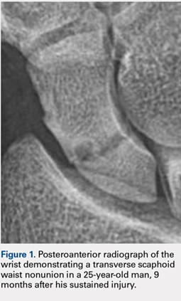
Of the 23 patients, 21 were found to have centrally placed variable compression screws based on Trumble and colleagues’8 criteria. Of the 23 patients, 19 had a complete follow-up course with radiographs at 6 months after surgery. All of these 19 patients had evidence of radiographic union defined as bridging trabeculation with near or complete obliteration of the fracture line on PA, lateral, and scaphoid radiographic views (Figure 2). Of the 6 smokers, 5 progressed to radiographic union and 1 patient had <6 months of postoperative return visits and could not be contacted. At the final clinic visit, all of the 19 patients denied wrist pain on direct palpation over the scaphoid tubercle, and no complications were reported. There were no repeat or revision surgical interventions.
Four patients had limited follow-up with <6 months of postoperative return visits. Their final set of radiographs did not demonstrate complete bridging trabeculation. One patient who moved away from the area was lost to follow-up but was contacted. The patient stated that he had a pain-free wrist with no further surgical interventions on his scaphoid. The other 3 patients could not be contacted.
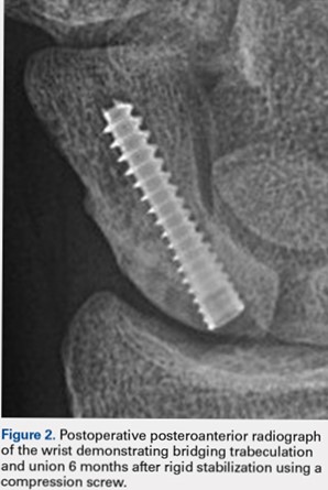
DISCUSSION
The management of scaphoid nonunions and delayed unions has dramatically evolved over the past 20 years.1,3-8 Historically, semi-rigid stabilization using Kirschner wires and casting afforded a 77% union rate in these cases.9 More recently, several authors have reported that stabilization without bone grafting can predictably unite scaphoid nonunions. Treating patients with uncomplicated scaphoid nonunions and delayed unions by internal fixation alone may be all that is required to achieve union.
The definitions of a scaphoid nonunion and delayed union are complex. The exact time when a scaphoid fracture heals varies between patients.2,5,10 However, the majority of hand surgeons believe that failure to see clear signs of healing (in waist fractures) after 3 months from the injury would suggest a failure to heal and a “delayed” union, whereas failure after 6 months from the injury and without clear signs of healing indicate a nonunion.5,6,10,11 Any resorption at the fracture site suggests that the fracture will not heal by continued immobilization alone and will require surgery.10
Continue to: Hand surgeons have several surgical options...
Hand surgeons have several surgical options when managing scaphoid injuries. Mahmoud and Koptan4 used a volar approach to percutaneously deliver a headless compression screw into 27 nonunions. Postoperative CT scans demonstrated fracture union in all 27 patients, and no patient underwent revision surgery. Interestingly, 14 of their patients had extensive preoperative resorption (but no deformity) of >5 mm.
Although volar percutaneous approaches for internal fixation have been cited to provide high rates of union and high patient satisfaction in acute scaphoid fracture fixation, this study utilized a dorsal approach. Both Wozasek and Moser12 and Haddad and Goddard13 reported excellent results and high union rates using a volar approach in consecutive acute scaphoid fractures. Despite these results, there are concerns that using a volar approach may damage the scaphotrapezial joint and may be prone to eccentric placement of compression screws.8,14
Slade and colleagues3 did utilize the dorsal approach with arthroscopic assistance to deliver a compression screw into scaphoid nonunions in 15 consecutive patients without any evidence of deformity, sclerosis, or resorption. Similar to our investigation, they treated patients with both delayed unions and nonunions. CT scans were used to confirm unions in all their patients. Using a dorsal approach, Yassaee and Yang15 treated 9 consecutive patients using a compression screw without bone grafting for both delayed and nonunion scaphoid injuries. Other authors have used both volar and dorsal approaches in 12 consecutive delayed and nonunion scaphoid injuries and found that 11 of the 12 injuries progressed to unions.6
Although these authors and several others advocate the use of CT scans to assess unions, our investigation used bridging trabeculation obliteration of the fracture line on 3 standard radiographic views to confirm unions in addition to the absence of pain clinically.16,17 CT scans expose the patient to increased radiation that, in our experience, does not alter the postoperative clinical course.18 If there is clear evidence of bridged callus and no pain on physical examination, a CT scan performed to reconfirm the union affords little benefit to clinical management.19
Continue to: All these previous studies have demonstrated...
All these previous studies have demonstrated excellent union rates but using a limited series of patients. We reviewed a large number of consecutive patients with scaphoid delayed unions and nonunions treated by screw fixation without bone grafting. Our hospital is a safety net institution for a large urban catchment area and had complete radiographic and clinical data for 19 of our 23 patients. One patient was contacted by telephone and he reported no pain and no revision surgical interventions.
The limitations of this study include not only its retrospective design but also its limited secondary outcome measures. However, our primary outcomes of union, pain, and complications are of utmost importance to clinicians and patients alike. Similar to other authors, we used radiographs to confirm unions. Although bridging trabeculation in radiographs has been demonstrated as soon as 1 month after the injury, there may be problems with interobserver reliability.4,13,15,20,21
Patients being lost to follow-up is not uncommon in the orthopedic trauma literature and can influence results.22,23 It is speculative to infer that the 3 patients who did not complete a follow-up course did not return because their pain had mitigated.
CONCLUSION
Like several fractures, the lack of stability and the absence of micro-motion are believed to contribute to fibrous nonunions in scaphoid fractures.13 This study provides a large consecutive cohort of patients with minimally displaced scaphoid delayed unions and nonunions that were successfully treated by rigid internal fixation without bone grafting. These results confirm previous reports that bone grafting is not required to provide predictable unions for the majority of scaphoid nonunions.
This paper will be judged for the Resident Writer’s Award.
1. Trumble TE, Salas P, Barthel T, Robert KQ 3rd. Management of scaphoid nonunions. J Am Acad Orthop Surg. 2003;11(6):380-391. doi:10.1016/j.jhsa.2012.03.002.
2. Munk B, Larsen CF. Bone grafting the scaphoid nonunion: a systematic review of 147 publications including 5,246 cases of scaphoid nonunion. Acta Orthop Scand. 2004;75(5):618-629. doi:10.1080/00016470410001529.
3. Slade JF 3rd, Geissler WB, Gutow AP, Merrell GA. Percutaneous internal fixation of selected scaphoid nonunions with an arthroscopically assisted dorsal approach. J Bone Joint Surg Am. 2003;85-A Suppl 4:20-32.
4. Mahmoud M, Koptan W. Percutaneous screw fixation without bone grafting for established scaphoid nonunion with substantial bone loss. J Bone Joint Surg Br. 2011;93(7):932-936. doi:10.1302/0301-620X.93B7.25418.
5. Inaparthy PK, Nicholl JE. Treatment of delayed/nonunion of scaphoid waist with Synthes cannulated scaphoid screw and bone graft. Hand N Y N. 2008;3(4):292-296. doi:10.1007/s11552-008-9112-4.
6. Capo JT, Shamian B, Rizzo M. Percutaneous screw fixation without bone grafting of scaphoid non-union. Isr Med Assoc J. 2012;14(12):729-732.
7. Kim JK, Kim JO, Lee SY. Volar percutaneous screw fixation for scaphoid waist delayed union. Clin Orthop Relat Res. 2010;468(4):1066-1071. doi:10.1007/s11999-009-1032-2.
8. Trumble TE, Clarke T, Kreder HJ. Non-union of the scaphoid. Treatment with cannulated screws compared with treatment with Herbert screws. J Bone Joint Surg Am. 1996;78(12):1829-1837.
9. Cosio MQ, Camp RA. Percutaneous pinning of symptomatic scaphoid nonunions. J Hand Surg. 1986;11(3):350-355. doi:10.1016/S0363-5023(86)80141-1.
10. Steinmann SP, Adams JE. Scaphoid fractures and nonunions: diagnosis and treatment. J Orthop Sci. 2006;11(4):424-431. doi:10.1007/s00776-006-1025-x.
11. Zarezadeh A, Moezi M, Rastegar S, Motififard M, Foladi A, Daneshpajouhnejad P. Scaphoid nonunion fracture and results of the modified Matti-Russe technique. Adv Biomed Res. 2015;4:39. doi:10.4103/2277-9175.151248.
12. Wozasek GE, Moser KD. Percutaneous screw fixation for fractures of the scaphoid. J Bone Joint Surg Br. 1991;73(1):138-142. doi:10.3928/01477447-20170509-04.
13. Haddad FS, Goddard NJ. Acute percutaneous scaphoid fixation. A pilot study. J Bone Joint Surg Br. 1998;80(1):95-99. doi:10.1302/0301-620X.80B1.8076.
14. Yip HSF, Wu WC, Chang RYP, So TYC. Percutaneous cannulated screw fixation of acute scaphoid waist fracture. J Hand Surg Br. 2002;27(1):42-46. doi:10.1054/jhsb.2001.0690.
15. Yassaee F, Yang SS. Mini-incision fixation of nondisplaced scaphoid fracture nonunions. J Hand Surg. 2008;33(7):1116-1120. doi:10.1016/j.jhsa.2008.03.004.
16. Slade JF 3rd, Gillon T. Retrospective review of 234 scaphoid fractures and nonunions treated with arthroscopy for union and complications. Scand J Surg. 2008;97(4):280-289. doi:10.1177/145749690809700402
17. Geoghegan JM, Woodruff MJ, Bhatia R, et al. Undisplaced scaphoid waist fractures: is 4 weeks’ immobilisation in a below-elbow cast sufficient if a week 4 CT scan suggests fracture union? J Hand Surg Eur Vol. 2009;34(5):631-637. doi:10.1177/1753193409105189.
18. Biswas D, Bible JE, Bohan M, Simpson AK, Whang PG, Grauer JN. Radiation exposure from musculoskeletal computerized tomographic scans. J Bone Joint Surg Am. 2009;91(8):1882-1889. doi:10.2106/JBJS.H.01199.
19. Dias JJ, Taylor M, Thompson J, Brenkel IJ, Gregg PJ. Radiographic signs of union of scaphoid fractures. An analysis of inter-observer agreement and reproducibility. J Bone Joint Surg Br. 1988;70(2):299-301. doi:10.1302/0301-620X.70B2.3346310.
20. Martus JE, Bedi A, Jebson PJL. Cannulated variable pitch compression screw fixation of scaphoid fractures using a limited dorsal approach. Tech Hand Up Extrem Surg. 2005;9(4):202-206. doi:10.1097/01.bth.0000191422.26565.25.
21. Clay NR, Dias JJ, Costigan PS, Gregg PJ, Barton NJ. Need the thumb be immobilised in scaphoid fractures? A randomised prospective trial. J Bone Joint Surg Br. 1991;73(5):828-832. doi:10.1302/0301-620X.73B5.1894676.
22. Zelle BA, Bhandari M, Sanchez AI, Probst C, Pape HC. Loss of follow-up in orthopaedic trauma: is 80% follow-up still acceptable? J Orthop Trauma. 2013;27(3):177-181. doi:10.1097/BOT.0b013e31825cf367.
23. Sprague S, Leece P, Bhandari M, et al. Limiting loss to follow-up in a multicenter randomized trial in orthopedic surgery. Control Clin Trials. 2003;24(6):719-725. doi:10.1016/j.cct.2003.08.012.
ABSTRACT
Delayed unions and nonunions of the scaphoid are most often treated by open reduction and internal fixation with bone grafting. We sought to evaluate a large consecutive series of nondisplaced or minimally displaced scaphoid nonunions and delayed unions treated by a compression screw without bone grafting by 2 fellowship trained hand surgeons. A total of 23 patients (19 males, 4 females) were identified who had fractures located at the distal third (2), the waist (18), and the proximal third (3). Of the 23 patients, 19 had a complete follow-up (mean follow-up period, 5.2 months) with evidence of radiographic union. There were no radiographic signs of arthrosis, osteonecrosis of the scaphoid, hardware-related complications, or reported revision surgeries. In conclusion, nonunions and delayed unions in nondisplaced or minimally displaced scaphoids without carpal malalignment can be successfully treated using compression screw fixation without bone grafting.
Continued to: Scaphoid nonunions or delayed unions with displacement...
Scaphoid nonunions or delayed unions with displacement, humpback deformities, or dorsal intercalated segmental instability deformities require open exposure with reduction of the fracture and autogenous bone grafting (structural or nonstructural and vascularized or nonvascularized).1,2 However, in the absence of displacement or deformity, compression and internal fixation without bone grafting may be sufficient to achieve union.
Several reports have described the use of internal fixation alone in the management of scaphoid nonunions with both minimal and extensive bone loss.3-7 These studies have shown that screw fixation alone affords less morbidity to the patient while allowing high rates of union.
Previous reports of internal fixation alone included limited numbers of patients for review. Therefore, we aim to review a large consecutive series of scaphoid delayed unions and nonunions without osteonecrosis or deformity managed by only internal fixation. Our hypothesis is that drilling combined with compression and rigid stabilization would allow for bony union in these cases
MATERIALS AND METHODS
After Institutional Review Board approval was obtained, a retrospective review of prospectively collected data was performed on consecutive patients with a delayed union or nonunion of the scaphoid. All injuries had failed conservative treatment of casting for at least 12 weeks and ultrasound stimulation, and were subsequently treated by compression screw fixation by 1 of 2 fellowship trained hand surgeons. The database comprised the data of patients who presented to a single, Level 1 trauma center between 2000 and 2012.
Delayed unions and nonunions were defined as a lack of radiographic trabecular bridging and pain on clinical examination at 3 and 6 months, respectively. All fractures were nondisplaced or minimally displaced (<2 mm), and patients with carpal malalignment or humpback deformity (based on scapholunate angle on plain radiographs) were excluded. Clinical outcome measures included evidence of radiographic union, revision surgery, pain, and reported complications.
Continue to: Inclusion criteria were all patients who sustained...
Inclusion criteria were all patients who sustained a minimally displaced scaphoid fracture and were treated conservatively with casting for at least 12 weeks and ultrasound stimulation, and progressed to delayed unions or nonunions.
Patients younger than age 18 years or with radiographic evidence of arthrosis or humpback deformity were excluded. Any fracture with >2 mm of gapping on original injury radiographs was not considered as minimally displaced and was also excluded. Furthermore, patients with a previous ipsilateral scaphoid injury or hand surgery were also excluded.
Compression screw placement was recorded as being either central or eccentric based on Trumble and colleagues’8 criteria. Posteroanterior (PA), lateral, and scaphoid view radiographs were reviewed by the first author (DS) and the treating hand surgeon (AS). Central screw placement was substantiated if the screw was in the middle third of the proximal pole in all 3 views.
The final set of postoperative radiographs was reviewed for unions. Union was defined as bridging trabeculation with near or complete obliteration of the fracture line on PA, lateral, and scaphoid radiographic views. Computerized tomography (CT) was performed at the discretion of the treating surgeon, and its use was not required if there was near obliteration of the fracture line on the 3-view radiographs and in the absence of patient-reported pain. Patients with bone loss or sclerosis were included as long as no deformity existed.
After surgical intervention, a short-arm cast was applied for 6 weeks, followed by a wrist splint for 4 to 8 weeks depending on patient comfort.
Continue to: SURGICAL TECHNIQUE...
SURGICAL TECHNIQUE
Either a 1-cm to 2-cm transverse incision distal to Lister’s tubercle or a longitudinal incision just ulnar was utilized. The extensor pollicis longus was identified and retracted. A longitudinal or an L-shaped capsulotomy was made to identify the proximal pole of the scaphoid. With the wrist flexed, a guide wire was inserted down the central axis of the scaphoid and confirmed by fluoroscopy. The measurement was made off the guidewire and 4 to 6 mm was subtracted. The scaphoid was then drilled, and the variable pitch compression screw (Acutrak Headless Compression Screw, Acumed) was inserted. Compression and position of the screw were confirmed by fluoroscopy before closure.
RESULTS
A total of 23 patients (19 males, 4 females) with acute scaphoid fractures who were treated conservatively with casting for at least 12 weeks and ultrasound stimulation, and progressed to delayed unions or nonunions were identified in this study. The ages of the patients ranged from 19 to 50 years. Of the 23 patients, 6 were smokers. The majority of patients sustained fractures in the scaphoid waist (18 patients) (Figure 1). Two patients had distal third fractures, and 3 had proximal third fractures.
The average time from the sustained injury to the surgical intervention was 8.2 months (range, 3.1-27.6 months). There were no patients with delayed diagnoses. Three fractures were identified as delayed unions with failure of union and pain after 3 months of conservative treatment, whereas the other 20 were identified as nonunions with at least 6 months of failed conservative treatment.
Of the 23 patients, 21 were found to have centrally placed variable compression screws based on Trumble and colleagues’8 criteria. Of the 23 patients, 19 had a complete follow-up course with radiographs at 6 months after surgery. All of these 19 patients had evidence of radiographic union defined as bridging trabeculation with near or complete obliteration of the fracture line on PA, lateral, and scaphoid radiographic views (Figure 2). Of the 6 smokers, 5 progressed to radiographic union and 1 patient had <6 months of postoperative return visits and could not be contacted. At the final clinic visit, all of the 19 patients denied wrist pain on direct palpation over the scaphoid tubercle, and no complications were reported. There were no repeat or revision surgical interventions.
Four patients had limited follow-up with <6 months of postoperative return visits. Their final set of radiographs did not demonstrate complete bridging trabeculation. One patient who moved away from the area was lost to follow-up but was contacted. The patient stated that he had a pain-free wrist with no further surgical interventions on his scaphoid. The other 3 patients could not be contacted.
DISCUSSION
The management of scaphoid nonunions and delayed unions has dramatically evolved over the past 20 years.1,3-8 Historically, semi-rigid stabilization using Kirschner wires and casting afforded a 77% union rate in these cases.9 More recently, several authors have reported that stabilization without bone grafting can predictably unite scaphoid nonunions. Treating patients with uncomplicated scaphoid nonunions and delayed unions by internal fixation alone may be all that is required to achieve union.
The definitions of a scaphoid nonunion and delayed union are complex. The exact time when a scaphoid fracture heals varies between patients.2,5,10 However, the majority of hand surgeons believe that failure to see clear signs of healing (in waist fractures) after 3 months from the injury would suggest a failure to heal and a “delayed” union, whereas failure after 6 months from the injury and without clear signs of healing indicate a nonunion.5,6,10,11 Any resorption at the fracture site suggests that the fracture will not heal by continued immobilization alone and will require surgery.10
Continue to: Hand surgeons have several surgical options...
Hand surgeons have several surgical options when managing scaphoid injuries. Mahmoud and Koptan4 used a volar approach to percutaneously deliver a headless compression screw into 27 nonunions. Postoperative CT scans demonstrated fracture union in all 27 patients, and no patient underwent revision surgery. Interestingly, 14 of their patients had extensive preoperative resorption (but no deformity) of >5 mm.
Although volar percutaneous approaches for internal fixation have been cited to provide high rates of union and high patient satisfaction in acute scaphoid fracture fixation, this study utilized a dorsal approach. Both Wozasek and Moser12 and Haddad and Goddard13 reported excellent results and high union rates using a volar approach in consecutive acute scaphoid fractures. Despite these results, there are concerns that using a volar approach may damage the scaphotrapezial joint and may be prone to eccentric placement of compression screws.8,14
Slade and colleagues3 did utilize the dorsal approach with arthroscopic assistance to deliver a compression screw into scaphoid nonunions in 15 consecutive patients without any evidence of deformity, sclerosis, or resorption. Similar to our investigation, they treated patients with both delayed unions and nonunions. CT scans were used to confirm unions in all their patients. Using a dorsal approach, Yassaee and Yang15 treated 9 consecutive patients using a compression screw without bone grafting for both delayed and nonunion scaphoid injuries. Other authors have used both volar and dorsal approaches in 12 consecutive delayed and nonunion scaphoid injuries and found that 11 of the 12 injuries progressed to unions.6
Although these authors and several others advocate the use of CT scans to assess unions, our investigation used bridging trabeculation obliteration of the fracture line on 3 standard radiographic views to confirm unions in addition to the absence of pain clinically.16,17 CT scans expose the patient to increased radiation that, in our experience, does not alter the postoperative clinical course.18 If there is clear evidence of bridged callus and no pain on physical examination, a CT scan performed to reconfirm the union affords little benefit to clinical management.19
Continue to: All these previous studies have demonstrated...
All these previous studies have demonstrated excellent union rates but using a limited series of patients. We reviewed a large number of consecutive patients with scaphoid delayed unions and nonunions treated by screw fixation without bone grafting. Our hospital is a safety net institution for a large urban catchment area and had complete radiographic and clinical data for 19 of our 23 patients. One patient was contacted by telephone and he reported no pain and no revision surgical interventions.
The limitations of this study include not only its retrospective design but also its limited secondary outcome measures. However, our primary outcomes of union, pain, and complications are of utmost importance to clinicians and patients alike. Similar to other authors, we used radiographs to confirm unions. Although bridging trabeculation in radiographs has been demonstrated as soon as 1 month after the injury, there may be problems with interobserver reliability.4,13,15,20,21
Patients being lost to follow-up is not uncommon in the orthopedic trauma literature and can influence results.22,23 It is speculative to infer that the 3 patients who did not complete a follow-up course did not return because their pain had mitigated.
CONCLUSION
Like several fractures, the lack of stability and the absence of micro-motion are believed to contribute to fibrous nonunions in scaphoid fractures.13 This study provides a large consecutive cohort of patients with minimally displaced scaphoid delayed unions and nonunions that were successfully treated by rigid internal fixation without bone grafting. These results confirm previous reports that bone grafting is not required to provide predictable unions for the majority of scaphoid nonunions.
This paper will be judged for the Resident Writer’s Award.
1. Trumble TE, Salas P, Barthel T, Robert KQ 3rd. Management of scaphoid nonunions. J Am Acad Orthop Surg. 2003;11(6):380-391. doi:10.1016/j.jhsa.2012.03.002.
2. Munk B, Larsen CF. Bone grafting the scaphoid nonunion: a systematic review of 147 publications including 5,246 cases of scaphoid nonunion. Acta Orthop Scand. 2004;75(5):618-629. doi:10.1080/00016470410001529.
3. Slade JF 3rd, Geissler WB, Gutow AP, Merrell GA. Percutaneous internal fixation of selected scaphoid nonunions with an arthroscopically assisted dorsal approach. J Bone Joint Surg Am. 2003;85-A Suppl 4:20-32.
4. Mahmoud M, Koptan W. Percutaneous screw fixation without bone grafting for established scaphoid nonunion with substantial bone loss. J Bone Joint Surg Br. 2011;93(7):932-936. doi:10.1302/0301-620X.93B7.25418.
5. Inaparthy PK, Nicholl JE. Treatment of delayed/nonunion of scaphoid waist with Synthes cannulated scaphoid screw and bone graft. Hand N Y N. 2008;3(4):292-296. doi:10.1007/s11552-008-9112-4.
6. Capo JT, Shamian B, Rizzo M. Percutaneous screw fixation without bone grafting of scaphoid non-union. Isr Med Assoc J. 2012;14(12):729-732.
7. Kim JK, Kim JO, Lee SY. Volar percutaneous screw fixation for scaphoid waist delayed union. Clin Orthop Relat Res. 2010;468(4):1066-1071. doi:10.1007/s11999-009-1032-2.
8. Trumble TE, Clarke T, Kreder HJ. Non-union of the scaphoid. Treatment with cannulated screws compared with treatment with Herbert screws. J Bone Joint Surg Am. 1996;78(12):1829-1837.
9. Cosio MQ, Camp RA. Percutaneous pinning of symptomatic scaphoid nonunions. J Hand Surg. 1986;11(3):350-355. doi:10.1016/S0363-5023(86)80141-1.
10. Steinmann SP, Adams JE. Scaphoid fractures and nonunions: diagnosis and treatment. J Orthop Sci. 2006;11(4):424-431. doi:10.1007/s00776-006-1025-x.
11. Zarezadeh A, Moezi M, Rastegar S, Motififard M, Foladi A, Daneshpajouhnejad P. Scaphoid nonunion fracture and results of the modified Matti-Russe technique. Adv Biomed Res. 2015;4:39. doi:10.4103/2277-9175.151248.
12. Wozasek GE, Moser KD. Percutaneous screw fixation for fractures of the scaphoid. J Bone Joint Surg Br. 1991;73(1):138-142. doi:10.3928/01477447-20170509-04.
13. Haddad FS, Goddard NJ. Acute percutaneous scaphoid fixation. A pilot study. J Bone Joint Surg Br. 1998;80(1):95-99. doi:10.1302/0301-620X.80B1.8076.
14. Yip HSF, Wu WC, Chang RYP, So TYC. Percutaneous cannulated screw fixation of acute scaphoid waist fracture. J Hand Surg Br. 2002;27(1):42-46. doi:10.1054/jhsb.2001.0690.
15. Yassaee F, Yang SS. Mini-incision fixation of nondisplaced scaphoid fracture nonunions. J Hand Surg. 2008;33(7):1116-1120. doi:10.1016/j.jhsa.2008.03.004.
16. Slade JF 3rd, Gillon T. Retrospective review of 234 scaphoid fractures and nonunions treated with arthroscopy for union and complications. Scand J Surg. 2008;97(4):280-289. doi:10.1177/145749690809700402
17. Geoghegan JM, Woodruff MJ, Bhatia R, et al. Undisplaced scaphoid waist fractures: is 4 weeks’ immobilisation in a below-elbow cast sufficient if a week 4 CT scan suggests fracture union? J Hand Surg Eur Vol. 2009;34(5):631-637. doi:10.1177/1753193409105189.
18. Biswas D, Bible JE, Bohan M, Simpson AK, Whang PG, Grauer JN. Radiation exposure from musculoskeletal computerized tomographic scans. J Bone Joint Surg Am. 2009;91(8):1882-1889. doi:10.2106/JBJS.H.01199.
19. Dias JJ, Taylor M, Thompson J, Brenkel IJ, Gregg PJ. Radiographic signs of union of scaphoid fractures. An analysis of inter-observer agreement and reproducibility. J Bone Joint Surg Br. 1988;70(2):299-301. doi:10.1302/0301-620X.70B2.3346310.
20. Martus JE, Bedi A, Jebson PJL. Cannulated variable pitch compression screw fixation of scaphoid fractures using a limited dorsal approach. Tech Hand Up Extrem Surg. 2005;9(4):202-206. doi:10.1097/01.bth.0000191422.26565.25.
21. Clay NR, Dias JJ, Costigan PS, Gregg PJ, Barton NJ. Need the thumb be immobilised in scaphoid fractures? A randomised prospective trial. J Bone Joint Surg Br. 1991;73(5):828-832. doi:10.1302/0301-620X.73B5.1894676.
22. Zelle BA, Bhandari M, Sanchez AI, Probst C, Pape HC. Loss of follow-up in orthopaedic trauma: is 80% follow-up still acceptable? J Orthop Trauma. 2013;27(3):177-181. doi:10.1097/BOT.0b013e31825cf367.
23. Sprague S, Leece P, Bhandari M, et al. Limiting loss to follow-up in a multicenter randomized trial in orthopedic surgery. Control Clin Trials. 2003;24(6):719-725. doi:10.1016/j.cct.2003.08.012.
TAKE-HOME POINTS
- Scaphoid nonunions can occur in minimally displaced fractures.
- If there is no deformity of the scaphoid delayed or nonunion, then a percutaneous screw fixation without bone grafting can reliably lead to bony union.
- Not all scaphoid delayed unions and nonunions require bone grafting.
Access to Transplant Care and Services Within the Veterans Health Administration
The Veterans Health Administration (VHA) provides health care services to over 9 million eligible and enrolled veterans out of a US veteran population of 18.9 million.1 In 2014, an Office of Inspector General (OIG) investigation identified timely access to health care within the VHA as a serious concern.2 In direct response, Congress enacted the Veterans Access, Choice, and Accountability Act (VACAA) of 2014 to expand access to care options available to veterans through referral to non-VA community care providers when the veteran is waiting longer than 30 days for an outpatient appointment or services, resides a significant distance (≥ 40 miles) from a VA facility, or experiences an undue burden to receive care and services.3 The VHA also responded, implementing several initiatives to improve veteran access to VHA health care generally, including the MyVA transformation and the proliferation of connected health technology; including telehealth capability and the expanded use of secure messaging. 4-6
This study examined veterans’ access to the VA transplant program (VATP) for fiscal year (FY 2014 to FY 2016). Timeliness of services and outcomes in relationship to the distance from a VA transplant center (VATC) were evaluated.
Methods
The VATP comprises the following VATCs: 5 heart (Madison, Wisconsin; Nashville, Tennessee; Palo Alto, California; Richmond, Virginia; and Salt Lake City, Utah); 7 kidney (Birmingham, Alabama; Bronx, New York; Houston, Texas; Iowa City, Iowa; Nashville, Tennessee; Pittsburgh, Pennsylvania; and Portland, Oregon); 6 liver (Houston, Texas; Madison, Wisconsin; Nashville, Tennessee; Pittsburgh, Pennsylvania; Portland, Oregon; and Richmond, Virginia); and 2 lung (Madison, Wisconsin; and Seattle, Washington).
In 2012, the VHA published a policy to establish timeliness standards for a VATC initial review decision and referral evaluation.7 In 2013, the VHA National Surgery Office (NSO) implemented a secure intranet-based application called TRACER to facilitate the referral process and track timeliness of initial review decision, evaluation, United Network of Organ Sharing (UNOS) waitlisting, and transplantation.
The referral process is as follows: The referring VA medical facility submits veteran candidate health information into TRACER, selects a VATC, and then TRACER notifies the VATC. The VATC reviews the information and submits an initial review decision as to whether the clinical information supports further evaluation within 48 hours for an emergency referral and 5 business days for a stable referral. If accepted, the VATC completes an evaluation within 30 calendar days of the referral submission date. On evaluation and acceptance, the VATC accepts handoff for transplant-related care, orders additional testing as needed, and waitlists the veteran with UNOS when the clinical status is deemed appropriate.4
The TRACER data from 3 separate cohorts were analyzed from October 1, 2013, to September 30, 2016, with a follow-up event capture through March 31, 2017: (1) the referral cohort, representing all referrals to the VATP; (2) the waitlist cohort, representing those undergoing initial UNOS waitlisting; and (3) the transplant cohort, representing those receiving a solid organ transplant. The straight-line distance between the referring VA medical facility and the VATC was determined for each referral and categorized as follows: less than 100 miles, 100 to 300 miles, 301 to 500 miles, and greater than 500 miles.
Mortality outcomes in the TRACER database were confirmed using the VHA Vital Status file, which combines the Centers for Medicare & Medicaid Services, Social Security Administration, and VHA internal utilization data to determine a best source, including flagging of records that indicate a death date followed by use of VA services.8,9 Records flagged with VA use after death were not considered deaths in this analysis. The NSO regularly refreshes veteran vital status information in the TRACER database for analysis of long-term outcomes.
The analysis methods for this study included Kruskall-Wallis nonparametric 1-way analysis of variance to compare timeliness metrics by distance group, Fine and Gray competing risks models to compare mortality on the UNOS list by distance group, and log-rank and Wilcoxon-Gehan tests to compare patient survival distributions by distance group.10-14 Analysis was generated using SAS software, version 9.4 (Cary, North Carolina) as well as the R statistical software application (r-project.org).15 Publicly available solid organ transplant survival rates were obtained from the Scientific Registry for Transplant Recipients (SRTR).16
Results
For FY 2014 to FY 2016, the referral cohort identified 6,009 veteran referrals to a VATC for solid organ transplant of which 3,500 underwent an evaluation, and 2,137 were waitlisted for solid organ transplant with UNOS (Table 1). 
For the study period, 6,009 referrals resulted in 188 emergency initial review decisions and 3,551 stable initial review decisions with an eligible declaration (Table 2). 

Three thousand five hundred evaluations were performed in a median time of 27 calendar days (IQR 21-32 d) with 948 (27.1%) performed beyond the policy mandated 30 calendar days. Telehealth was used for 555 evaluations (15.9%), primarily for referrals located greater than 100 miles from the VATC. In FY 2016, 13.1% of the 1,321 completed evaluations were performed beyond 30 calendar days, representing an improvement from prior years; 45.7% beyond 30 calendar days in FY 2014 and 26.2% beyond 30 days in FY 2015.
Of the 6,009 referrals submitted in FY 2014 to FY 2016, 2,137 were waitlisted with UNOS. The median time from referral to waitlisting was 78 calendar days (IQR 43-148 d) for the entire study period, decreasing from 90 calendar days in FY 2014 to 70 calendar days in FY 2016.
For all organs and most organ types, the time from referral to initial review decision, evaluation, and waitlisting was statistically less (P < .005) for referrals received from VA medical facilities located less than 100 miles compared with referrals received from VA medical facilities at least 100 miles from the VATC. No statistical difference was found for emergency initial review decision for heart (P = .72) and lung (P = .14), time to evaluation for lung (P = .14), and time to waitlisting for heart (P = .95).
The waitlist cohort data are shown in Table 3. 

TRACER identified that 339 (15.0%) of the waitlist cohort were removed from the UNOS waitlist of which 212 (62.5%) were removed for failure to meet clinical criteria for transplantation, and 127 (37.5%) were removed for patient choice. Overall, 226 (10.0%) veterans died during the study period without receiving a transplant. Organ-specific mortality rates for veterans waitlisted but not transplanted at a VATC are as follows: heart 6.1%, kidney 5.9%, liver 19.0%, and lung 11.5%. As of March 31, 2017, 1,051 veterans were waitlisted with UNOS of which 876 (83.3%) were waitlisted for a kidney transplant.
The rate of mortality on the UNOS waitlist, the percentage of veterans transplanted, the time from waitlisting to transplantation, and the percentage of patients waitlisted at the end of the study period were not statistically different for referrals less than 100 miles compared with referrals at least 100 miles for all organs or kidney and liver separately (P ≤ .05). The relatively small numbers of veterans waitlisted for heart and lung transplants and nominal mortality events precluded making statements regarding significance for waitlist mortality.
The transplant cohort comprised 947 veterans receiving a solid organ transplant, including 102 (10.8%) heart, 411 (43.4%) kidney, 383 (40.4%) liver, and 51 (5.4%) lung transplants (Table 4). 
The transplant 30-day, 180-day, and 1-year survival rates are shown in Table 5. 
Discussion
This study shows that the VATP delivers timely, high-quality care and services even when the veteran’s referring VA medical facility is located a considerable distance from the VATC. Three separate cohorts of veterans were examined for the FY 2014 to FY 2016 study period: those referred, those waitlisted, and those transplanted. The referral cohort identified 6,009 referral submissions, performed 3,500 evaluations on veterans deemed to be potential candidates for solid organ transplantation, and placed 2,137 of these referrals on the UNOS waitlist. The median time from referral to initial review decision was 5 hours for emergency referrals and 3 business days for stable referrals. The median time from referral to evaluation was 27 calendar days, and the median time from referral to UNOS waitlisting was 78 calendar days. Improvements in timeliness for referral initial review decision, evaluation completion, and waitlisting over the study period were reflective of VHA and NSO efforts to enhance access to services. In FY 2016, 100% of emergency referrals received an initial review decision within 48 hours, 91.4% of stable reviews received an initial review decision within 5 business days, and 86.9% of all referrals underwent evaluation within 30 calendar days.
Distance of less than 100 miles between the referring VA medical facility and the VATC was associated with statistically significant shorter times for initial review decision, evaluation, and UNOS waitlisting. Referrals from less than 100 miles were a minority (9.6%) of referrals and most often represented a direct referral from the VATC to its own program. Timeliness of referral initial review decision, evaluation, or UNOS waitlisting was similar for distance categories greater than 100 miles: 100 to 300 miles, 301 to 500 miles, or greater than 500 miles.
The waitlist cohort identified 2,265 veterans, of which 731 (32.3%) underwent transplantation and 226 (10.0%) died. All-cause mortality for veterans once waitlisted, whether or not maintained on the UNOS waitlist, varied among organs and was found to be 6.1% for heart, 5.9% for kidney, 19.0% for liver, and 11.5% for lung. Waitlist mortality and the time from referral to solid organ transplant was similar for all distance categories.
The transplant cohort identified 947 veterans receiving a solid organ transplant with a median time from referral to transplant that varied considerably by organ type; 301 days (10.0 mo) for heart transplants, 914 days (30.5 mo) for kidney transplants, 236 days (7.9 mo) for liver transplants, and 246 days (8.2 mo) for lung transplants. Time to transplant and posttransplant survival were similar in all distance categories. Moreover, the VATP 1-year survival rates compared favorably with published SRTR data.
Prior studies have shown that distance to a transplant center adversely impacts access to transplant services, mortality on the UNOS waitlist, and transplant outcomes.17-21 Patients living in small towns and isolated rural regions were 8% to 15% less likely to be waitlisted and 10% to 20% less likely to undergo heart, kidney, and liver transplantation than were patients in urban environments.17 This study found that a referral to the VATP from a VA medical facility located less than 100 miles from the VATC received an evaluation 5 to 7 days sooner and be placed on the UNOS waitlist 21 to 29 days sooner than a veteran referred to a VATC located at least 100 miles away. Contrary to prior studies, the distance from the VATC did not have an adverse impact on UNOS waitlist mortality, time to transplantation, or survival outcomes posttransplant.
The VHA offers a number of advantages to the veteran in need of transplant care and services. The VHA is the largest integrated health care system in the US designed specifically for veterans and their complex and specific needs with greater than 1,200 points of care and a single electronic health record optimizing coordinated services.22 In addition, the VHA’s use of telehealth to expedite evaluations and follow-up transplant care closer to home thereby obviating the need for travel. The VHA also has an electronic process to facilitate referral and tracking of timeliness of care (TRACER). Finally, VHA has policies that supports travel benefits, including lodging for the veteran, caregiver, and living donor if applicable for evaluations, transplant procedures, and follow-up care.4,23
The coordination of health care services in a single integrated health care system may be the most significant advantage.24 Multiple studies have examined dual care, representing care and services provided across 2 separate health care systems, showing an association between dual care and an increased risk of hospitalization, duplication of tests, rates for prescribing potentially unsafe medications, and mortality.25-27 Although no study to date is on point, it is reasonable to imply that dual care imposes unnecessary risks to the veteran receiving complex lifelong transplant care when the VATP is shown to provide timely and high-quality care.
Limitations
The retrospective design and limited study period represent limitations. Specifically, survival outcomes for veterans transplanted were limited to 1 year and do not rule out the possibility that distance to a VATC will impact survival rates at 3 and 5 years posttransplant.
Conclusion
A referral distance of less than 100 miles from the VATC most often represents a direct referral and is a factor in timeliness of transplant initial review decision, evaluation, and placement of the veteran on the UNOS waitlist. Distance between the referring VA medical facility and the VATC, including distances of greater than 500 miles, was not found to impact the rate of mortality on the UNOS waitlist, time to transplantation, or posttransplant survival. Overall, the VHA provides timely solid organ transplant care and services with outcomes comparable to that of nationally reported SRTR estimates. Future studies should examine the timeliness of services, outcomes, and costs associated with those veterans authorized by the VHA for non-VA community care and those veterans who independently elect to receive transplant care and services by a non-VA transplant center and return to the VHA for dual care following transplantation.
1. US Department of Veterans Affairs, National Center for VeteransAnalysis and Statistics. Profile of veterans: 2015: data from the American Community Survey. https://www.va.gov/VETDATA/DOCS/SPECIALREPORTS/PROFILE_OF_VETERANS_2015.PDF. Published March 2017. Accessed July 2, 2018.
2. US Department of Veterans Affairs, Office of the Inspector General. Review of alleged patient deaths, patient wait times, and scheduling practices at the Phoenix VA Health Care System. https://www.va.gov/OIG/PUBS/VAOIG-14-02603-267.PDF. Published August 26, 2014. Accessed July 2, 2018.
3. US Department of Veterans Affairs. VHA directive 1700: Veterans Choice Program. https://www.va.gov/VHAPUBLICATIONS/VIEWPUBLICATION.ASP?PUB_ID=3287. Published October 25, 2016. Accessed July 2, 2018.
4. US Department of Veterans Affairs. MyVA. https://www.va.gov/MYVA. Updated November 8, 2016. Accessed July 2, 2018.
5. US Department of Veterans Affairs. Telehealth services. https://www.telehealth.va.gov. Updated March 27, 2017. Accessed July 2, 2018.
6. US Department of Veterans Affairs. Secure messaging. My HealtheVet. https://www.myhealth.va.gov/MHV-PORTAL-WEB/SECURE-MESSAGING-SPOTLIGHT. Updated July 1, 2016. Accessed July 2, 2018.
7. US Department of Veterans Affairs, Veterans Health Administration. VHA directive 2012-018: Solid organ and bone marrow transplantation. Published July 9, 2012.
8. Page WF, Mahan CM, Kang HK. Vital status ascertainment through the files of the Department of Veterans Affairs and the Social Security Administration. Ann Epidemiol. 1996;6(2):102-109.
9. Sohn M-W, Arnold N, Maynard C, Hynes DM. Accuracy and completeness of mortality data in the Department of Veterans Affairs. Popul Health Metr. 2006;4:2.
10. Kruskal WH, Wallis WA. Use of ranks in one-criterion variance analysis. J Am Stat Assoc. 1952;47(260):583-621.
11. Fine JP, Gray RJ. A proportional hazards model for the subdistribution of a competing risk. J Am Stat Assoc. 1999;94(446):496-509.
12. Peto R, Peto J. Asymptotically efficient rank invariant test procedures. J R Stat Soc Ser A Stat Soc. 1972;135(2):185-207.
13. Gehan EA. A generalized Wilcoxon test for comparing arbitrarily singly-censored samples. Biometrika. 1965;52(1/2):203-223.
14. Lee ET, Desu MM, Gehan EA. A Monte Carlo study of the power of some two-sample tests. Biometrika. 1975;62(2):425-432.
15. The R Foundation. The R project for statistical computing. https://www.r-project.org. Accessed July 2, 2018.
16. Scientific Registry of Transplant Recipients. https://www.srtr.org. Accessed July 2, 2018.
17. Axelrod DA, Guidinger MK, Finlayson S, et al. Rates of solid-organ wait-listing, transplantation, and survival among residents of rural and urban areas. JAMA. 2008;299(2):202-207.
18. Thabut G, Munson J, Haynes K, Harhay MO, Christie JD, Halpern SD. Geographic disparities in access to lung transplantation before and after implementation of the lung allocation score. Am J Transplant. 2012;12(11):3085-3093.
19. Zorzi D, Rastellini C, Freeman DH, Elias G, Duchini A, Cicalese L. Increase in mortality rate of liver transplant candidates residing in specific geographic areas: analysis of UNOS data. Am J Transplant. 2012;12(8):2188-2197.
20. Goldberg DS, French B, Forde KA, et al. Association of distance from a transplant center with access to waitlist placement, receipt of liver transplantation, and survival among US veterans. JAMA. 2014;311(12):1234-1243.
21. Cicalese L, Shirafkan A, Jennings K, Zorzi D, Rastellini C. Increased risk of death for patients on the waitlist for liver transplant residing at greater distance from specialized liver transplant centers in the United States. Transplantation. 2016;100(10):2146-2152.
22. US Department of Veterans Affairs. About VHA. https://www.va.gov/health/aboutvha.asp. Updated March 19, 2018. Accessed July 5, 2018.
23. US Department of Veterans Affairs, Veterans Health Administration. Veterans Health Administration handbook 1601B.05: beneficiary travel. https://www.va.gov/vhapublications/ViewPublication.asp?pub_ID=2275. Published July 21, 2010. Accessed July 5, 2018.
24. Gellad WF. The Veterans Choice Act and dual health system use. J Gen Intern Med. 2016;31(2):153-154.
25. Kothari AN, Loy VM, Brownlee SA, et al. Adverse effect of post-discharge care fragmentation on outcomes after readmissions after liver transplantation. J Am Coll Surg. 2017;225(1):62-67.
26. Thorpe JM, Thorpe CT, Gellad WF, et al. Dual health care system use and high-risk prescribing in patients with dementia. Ann Int Med. 2017;166(3):157-163.
27. Tarlov E, Lee TA, Weichle TW, et al. Reduced overall and event-free survival among colon cancer patients using dual system care. Cancer Epidemiol Biomarkers Prev. 2012;21(12):2231-2241.
The Veterans Health Administration (VHA) provides health care services to over 9 million eligible and enrolled veterans out of a US veteran population of 18.9 million.1 In 2014, an Office of Inspector General (OIG) investigation identified timely access to health care within the VHA as a serious concern.2 In direct response, Congress enacted the Veterans Access, Choice, and Accountability Act (VACAA) of 2014 to expand access to care options available to veterans through referral to non-VA community care providers when the veteran is waiting longer than 30 days for an outpatient appointment or services, resides a significant distance (≥ 40 miles) from a VA facility, or experiences an undue burden to receive care and services.3 The VHA also responded, implementing several initiatives to improve veteran access to VHA health care generally, including the MyVA transformation and the proliferation of connected health technology; including telehealth capability and the expanded use of secure messaging. 4-6
This study examined veterans’ access to the VA transplant program (VATP) for fiscal year (FY 2014 to FY 2016). Timeliness of services and outcomes in relationship to the distance from a VA transplant center (VATC) were evaluated.
Methods
The VATP comprises the following VATCs: 5 heart (Madison, Wisconsin; Nashville, Tennessee; Palo Alto, California; Richmond, Virginia; and Salt Lake City, Utah); 7 kidney (Birmingham, Alabama; Bronx, New York; Houston, Texas; Iowa City, Iowa; Nashville, Tennessee; Pittsburgh, Pennsylvania; and Portland, Oregon); 6 liver (Houston, Texas; Madison, Wisconsin; Nashville, Tennessee; Pittsburgh, Pennsylvania; Portland, Oregon; and Richmond, Virginia); and 2 lung (Madison, Wisconsin; and Seattle, Washington).
In 2012, the VHA published a policy to establish timeliness standards for a VATC initial review decision and referral evaluation.7 In 2013, the VHA National Surgery Office (NSO) implemented a secure intranet-based application called TRACER to facilitate the referral process and track timeliness of initial review decision, evaluation, United Network of Organ Sharing (UNOS) waitlisting, and transplantation.
The referral process is as follows: The referring VA medical facility submits veteran candidate health information into TRACER, selects a VATC, and then TRACER notifies the VATC. The VATC reviews the information and submits an initial review decision as to whether the clinical information supports further evaluation within 48 hours for an emergency referral and 5 business days for a stable referral. If accepted, the VATC completes an evaluation within 30 calendar days of the referral submission date. On evaluation and acceptance, the VATC accepts handoff for transplant-related care, orders additional testing as needed, and waitlists the veteran with UNOS when the clinical status is deemed appropriate.4
The TRACER data from 3 separate cohorts were analyzed from October 1, 2013, to September 30, 2016, with a follow-up event capture through March 31, 2017: (1) the referral cohort, representing all referrals to the VATP; (2) the waitlist cohort, representing those undergoing initial UNOS waitlisting; and (3) the transplant cohort, representing those receiving a solid organ transplant. The straight-line distance between the referring VA medical facility and the VATC was determined for each referral and categorized as follows: less than 100 miles, 100 to 300 miles, 301 to 500 miles, and greater than 500 miles.
Mortality outcomes in the TRACER database were confirmed using the VHA Vital Status file, which combines the Centers for Medicare & Medicaid Services, Social Security Administration, and VHA internal utilization data to determine a best source, including flagging of records that indicate a death date followed by use of VA services.8,9 Records flagged with VA use after death were not considered deaths in this analysis. The NSO regularly refreshes veteran vital status information in the TRACER database for analysis of long-term outcomes.
The analysis methods for this study included Kruskall-Wallis nonparametric 1-way analysis of variance to compare timeliness metrics by distance group, Fine and Gray competing risks models to compare mortality on the UNOS list by distance group, and log-rank and Wilcoxon-Gehan tests to compare patient survival distributions by distance group.10-14 Analysis was generated using SAS software, version 9.4 (Cary, North Carolina) as well as the R statistical software application (r-project.org).15 Publicly available solid organ transplant survival rates were obtained from the Scientific Registry for Transplant Recipients (SRTR).16
Results
For FY 2014 to FY 2016, the referral cohort identified 6,009 veteran referrals to a VATC for solid organ transplant of which 3,500 underwent an evaluation, and 2,137 were waitlisted for solid organ transplant with UNOS (Table 1).
For the study period, 6,009 referrals resulted in 188 emergency initial review decisions and 3,551 stable initial review decisions with an eligible declaration (Table 2).
Three thousand five hundred evaluations were performed in a median time of 27 calendar days (IQR 21-32 d) with 948 (27.1%) performed beyond the policy mandated 30 calendar days. Telehealth was used for 555 evaluations (15.9%), primarily for referrals located greater than 100 miles from the VATC. In FY 2016, 13.1% of the 1,321 completed evaluations were performed beyond 30 calendar days, representing an improvement from prior years; 45.7% beyond 30 calendar days in FY 2014 and 26.2% beyond 30 days in FY 2015.
Of the 6,009 referrals submitted in FY 2014 to FY 2016, 2,137 were waitlisted with UNOS. The median time from referral to waitlisting was 78 calendar days (IQR 43-148 d) for the entire study period, decreasing from 90 calendar days in FY 2014 to 70 calendar days in FY 2016.
For all organs and most organ types, the time from referral to initial review decision, evaluation, and waitlisting was statistically less (P < .005) for referrals received from VA medical facilities located less than 100 miles compared with referrals received from VA medical facilities at least 100 miles from the VATC. No statistical difference was found for emergency initial review decision for heart (P = .72) and lung (P = .14), time to evaluation for lung (P = .14), and time to waitlisting for heart (P = .95).
The waitlist cohort data are shown in Table 3.
TRACER identified that 339 (15.0%) of the waitlist cohort were removed from the UNOS waitlist of which 212 (62.5%) were removed for failure to meet clinical criteria for transplantation, and 127 (37.5%) were removed for patient choice. Overall, 226 (10.0%) veterans died during the study period without receiving a transplant. Organ-specific mortality rates for veterans waitlisted but not transplanted at a VATC are as follows: heart 6.1%, kidney 5.9%, liver 19.0%, and lung 11.5%. As of March 31, 2017, 1,051 veterans were waitlisted with UNOS of which 876 (83.3%) were waitlisted for a kidney transplant.
The rate of mortality on the UNOS waitlist, the percentage of veterans transplanted, the time from waitlisting to transplantation, and the percentage of patients waitlisted at the end of the study period were not statistically different for referrals less than 100 miles compared with referrals at least 100 miles for all organs or kidney and liver separately (P ≤ .05). The relatively small numbers of veterans waitlisted for heart and lung transplants and nominal mortality events precluded making statements regarding significance for waitlist mortality.
The transplant cohort comprised 947 veterans receiving a solid organ transplant, including 102 (10.8%) heart, 411 (43.4%) kidney, 383 (40.4%) liver, and 51 (5.4%) lung transplants (Table 4).
The transplant 30-day, 180-day, and 1-year survival rates are shown in Table 5.
Discussion
This study shows that the VATP delivers timely, high-quality care and services even when the veteran’s referring VA medical facility is located a considerable distance from the VATC. Three separate cohorts of veterans were examined for the FY 2014 to FY 2016 study period: those referred, those waitlisted, and those transplanted. The referral cohort identified 6,009 referral submissions, performed 3,500 evaluations on veterans deemed to be potential candidates for solid organ transplantation, and placed 2,137 of these referrals on the UNOS waitlist. The median time from referral to initial review decision was 5 hours for emergency referrals and 3 business days for stable referrals. The median time from referral to evaluation was 27 calendar days, and the median time from referral to UNOS waitlisting was 78 calendar days. Improvements in timeliness for referral initial review decision, evaluation completion, and waitlisting over the study period were reflective of VHA and NSO efforts to enhance access to services. In FY 2016, 100% of emergency referrals received an initial review decision within 48 hours, 91.4% of stable reviews received an initial review decision within 5 business days, and 86.9% of all referrals underwent evaluation within 30 calendar days.
Distance of less than 100 miles between the referring VA medical facility and the VATC was associated with statistically significant shorter times for initial review decision, evaluation, and UNOS waitlisting. Referrals from less than 100 miles were a minority (9.6%) of referrals and most often represented a direct referral from the VATC to its own program. Timeliness of referral initial review decision, evaluation, or UNOS waitlisting was similar for distance categories greater than 100 miles: 100 to 300 miles, 301 to 500 miles, or greater than 500 miles.
The waitlist cohort identified 2,265 veterans, of which 731 (32.3%) underwent transplantation and 226 (10.0%) died. All-cause mortality for veterans once waitlisted, whether or not maintained on the UNOS waitlist, varied among organs and was found to be 6.1% for heart, 5.9% for kidney, 19.0% for liver, and 11.5% for lung. Waitlist mortality and the time from referral to solid organ transplant was similar for all distance categories.
The transplant cohort identified 947 veterans receiving a solid organ transplant with a median time from referral to transplant that varied considerably by organ type; 301 days (10.0 mo) for heart transplants, 914 days (30.5 mo) for kidney transplants, 236 days (7.9 mo) for liver transplants, and 246 days (8.2 mo) for lung transplants. Time to transplant and posttransplant survival were similar in all distance categories. Moreover, the VATP 1-year survival rates compared favorably with published SRTR data.
Prior studies have shown that distance to a transplant center adversely impacts access to transplant services, mortality on the UNOS waitlist, and transplant outcomes.17-21 Patients living in small towns and isolated rural regions were 8% to 15% less likely to be waitlisted and 10% to 20% less likely to undergo heart, kidney, and liver transplantation than were patients in urban environments.17 This study found that a referral to the VATP from a VA medical facility located less than 100 miles from the VATC received an evaluation 5 to 7 days sooner and be placed on the UNOS waitlist 21 to 29 days sooner than a veteran referred to a VATC located at least 100 miles away. Contrary to prior studies, the distance from the VATC did not have an adverse impact on UNOS waitlist mortality, time to transplantation, or survival outcomes posttransplant.
The VHA offers a number of advantages to the veteran in need of transplant care and services. The VHA is the largest integrated health care system in the US designed specifically for veterans and their complex and specific needs with greater than 1,200 points of care and a single electronic health record optimizing coordinated services.22 In addition, the VHA’s use of telehealth to expedite evaluations and follow-up transplant care closer to home thereby obviating the need for travel. The VHA also has an electronic process to facilitate referral and tracking of timeliness of care (TRACER). Finally, VHA has policies that supports travel benefits, including lodging for the veteran, caregiver, and living donor if applicable for evaluations, transplant procedures, and follow-up care.4,23
The coordination of health care services in a single integrated health care system may be the most significant advantage.24 Multiple studies have examined dual care, representing care and services provided across 2 separate health care systems, showing an association between dual care and an increased risk of hospitalization, duplication of tests, rates for prescribing potentially unsafe medications, and mortality.25-27 Although no study to date is on point, it is reasonable to imply that dual care imposes unnecessary risks to the veteran receiving complex lifelong transplant care when the VATP is shown to provide timely and high-quality care.
Limitations
The retrospective design and limited study period represent limitations. Specifically, survival outcomes for veterans transplanted were limited to 1 year and do not rule out the possibility that distance to a VATC will impact survival rates at 3 and 5 years posttransplant.
Conclusion
A referral distance of less than 100 miles from the VATC most often represents a direct referral and is a factor in timeliness of transplant initial review decision, evaluation, and placement of the veteran on the UNOS waitlist. Distance between the referring VA medical facility and the VATC, including distances of greater than 500 miles, was not found to impact the rate of mortality on the UNOS waitlist, time to transplantation, or posttransplant survival. Overall, the VHA provides timely solid organ transplant care and services with outcomes comparable to that of nationally reported SRTR estimates. Future studies should examine the timeliness of services, outcomes, and costs associated with those veterans authorized by the VHA for non-VA community care and those veterans who independently elect to receive transplant care and services by a non-VA transplant center and return to the VHA for dual care following transplantation.
1. US Department of Veterans Affairs, National Center for VeteransAnalysis and Statistics. Profile of veterans: 2015: data from the American Community Survey. https://www.va.gov/VETDATA/DOCS/SPECIALREPORTS/PROFILE_OF_VETERANS_2015.PDF. Published March 2017. Accessed July 2, 2018.
2. US Department of Veterans Affairs, Office of the Inspector General. Review of alleged patient deaths, patient wait times, and scheduling practices at the Phoenix VA Health Care System. https://www.va.gov/OIG/PUBS/VAOIG-14-02603-267.PDF. Published August 26, 2014. Accessed July 2, 2018.
3. US Department of Veterans Affairs. VHA directive 1700: Veterans Choice Program. https://www.va.gov/VHAPUBLICATIONS/VIEWPUBLICATION.ASP?PUB_ID=3287. Published October 25, 2016. Accessed July 2, 2018.
4. US Department of Veterans Affairs. MyVA. https://www.va.gov/MYVA. Updated November 8, 2016. Accessed July 2, 2018.
5. US Department of Veterans Affairs. Telehealth services. https://www.telehealth.va.gov. Updated March 27, 2017. Accessed July 2, 2018.
6. US Department of Veterans Affairs. Secure messaging. My HealtheVet. https://www.myhealth.va.gov/MHV-PORTAL-WEB/SECURE-MESSAGING-SPOTLIGHT. Updated July 1, 2016. Accessed July 2, 2018.
7. US Department of Veterans Affairs, Veterans Health Administration. VHA directive 2012-018: Solid organ and bone marrow transplantation. Published July 9, 2012.
8. Page WF, Mahan CM, Kang HK. Vital status ascertainment through the files of the Department of Veterans Affairs and the Social Security Administration. Ann Epidemiol. 1996;6(2):102-109.
9. Sohn M-W, Arnold N, Maynard C, Hynes DM. Accuracy and completeness of mortality data in the Department of Veterans Affairs. Popul Health Metr. 2006;4:2.
10. Kruskal WH, Wallis WA. Use of ranks in one-criterion variance analysis. J Am Stat Assoc. 1952;47(260):583-621.
11. Fine JP, Gray RJ. A proportional hazards model for the subdistribution of a competing risk. J Am Stat Assoc. 1999;94(446):496-509.
12. Peto R, Peto J. Asymptotically efficient rank invariant test procedures. J R Stat Soc Ser A Stat Soc. 1972;135(2):185-207.
13. Gehan EA. A generalized Wilcoxon test for comparing arbitrarily singly-censored samples. Biometrika. 1965;52(1/2):203-223.
14. Lee ET, Desu MM, Gehan EA. A Monte Carlo study of the power of some two-sample tests. Biometrika. 1975;62(2):425-432.
15. The R Foundation. The R project for statistical computing. https://www.r-project.org. Accessed July 2, 2018.
16. Scientific Registry of Transplant Recipients. https://www.srtr.org. Accessed July 2, 2018.
17. Axelrod DA, Guidinger MK, Finlayson S, et al. Rates of solid-organ wait-listing, transplantation, and survival among residents of rural and urban areas. JAMA. 2008;299(2):202-207.
18. Thabut G, Munson J, Haynes K, Harhay MO, Christie JD, Halpern SD. Geographic disparities in access to lung transplantation before and after implementation of the lung allocation score. Am J Transplant. 2012;12(11):3085-3093.
19. Zorzi D, Rastellini C, Freeman DH, Elias G, Duchini A, Cicalese L. Increase in mortality rate of liver transplant candidates residing in specific geographic areas: analysis of UNOS data. Am J Transplant. 2012;12(8):2188-2197.
20. Goldberg DS, French B, Forde KA, et al. Association of distance from a transplant center with access to waitlist placement, receipt of liver transplantation, and survival among US veterans. JAMA. 2014;311(12):1234-1243.
21. Cicalese L, Shirafkan A, Jennings K, Zorzi D, Rastellini C. Increased risk of death for patients on the waitlist for liver transplant residing at greater distance from specialized liver transplant centers in the United States. Transplantation. 2016;100(10):2146-2152.
22. US Department of Veterans Affairs. About VHA. https://www.va.gov/health/aboutvha.asp. Updated March 19, 2018. Accessed July 5, 2018.
23. US Department of Veterans Affairs, Veterans Health Administration. Veterans Health Administration handbook 1601B.05: beneficiary travel. https://www.va.gov/vhapublications/ViewPublication.asp?pub_ID=2275. Published July 21, 2010. Accessed July 5, 2018.
24. Gellad WF. The Veterans Choice Act and dual health system use. J Gen Intern Med. 2016;31(2):153-154.
25. Kothari AN, Loy VM, Brownlee SA, et al. Adverse effect of post-discharge care fragmentation on outcomes after readmissions after liver transplantation. J Am Coll Surg. 2017;225(1):62-67.
26. Thorpe JM, Thorpe CT, Gellad WF, et al. Dual health care system use and high-risk prescribing in patients with dementia. Ann Int Med. 2017;166(3):157-163.
27. Tarlov E, Lee TA, Weichle TW, et al. Reduced overall and event-free survival among colon cancer patients using dual system care. Cancer Epidemiol Biomarkers Prev. 2012;21(12):2231-2241.
Tranexamic Acid Reduces Perioperative Blood Loss and Hemarthrosis in Total Ankle Arthroplasty
ABSTRACT
Tranexamic acid (TXA) is an effective agent used for reducing perioperative blood loss and decreasing the potential for postoperative hemarthrosis. We hypothesized that patients who had received intraoperative TXA during total ankle arthroplasty (TAA) would have a reduction in postoperative drain output, thereby resulting in a reduced risk of postoperative hemarthrosis and lower wound complication rates.
A retrospective review was conducted on 50 consecutive patients, 25 receiving TXA (TXA-TAA) and 25 not receiving TXA (No TXA-TAA), who underwent an uncemented TAA between September 2011 and December 2015. Demographic characteristics, drain output, preoperative and postoperative hemoglobin levels, operative and postoperative course, and minor and major wound complications of the patients were reviewed.
Drain output was significantly less in the TXA-TAA group compared to that in the No TXA-TAA group (71.6 ± 60.3 vs 200.2 ± 117.0 mL, respectively, P < .0001). The overall wound complication rate in the No TXA-TAA group was higher (20%, 5/25) than that in the TXA-TAA group (8%, 2/25) (P = .114). The mean change in preoperative to postoperative hemoglobin level was significantly less in the TXA-TAA group compared to that in the No TXA-TAA group (1.5 ± 0.6 vs 2.0 ± 0.4 g/dL, respectively, P = .01).
TXA is an effective hemostatic agent when used during TAA. TXA reduces perioperative blood loss, hemarthrosis, and the risk of wound complications.
Continue to: End-stage ankle arthritis...
End-stage ankle arthritis is a disabling condition that may lead to poor quality of life and difficulties with activities of daily living.1 The associated mental and physical disability has been demonstrated to be as severe as in end-stage hip arthrosis.2 Operative treatment for symptomatic end-stage ankle arthritis includes arthrodesis or total ankle arthroplasty (TAA) in those refractory to nonoperative treatment.3 Newer generation implants have made TAA a more attractive option for both the surgeon and the patient.
Over the past decade, the utility of TAA has increased and attention has turned toward the management of perioperative factors that would maximize patient satisfaction and decrease the length of stay and complication rates, as well as hospital costs.4 Comprehensive literature on total knee arthroplasty (TKA) and total hip arthroplasty (THA) has demonstrated that the management of perioperative blood loss, specifically postoperative hemarthrosis, is a modifiable factor affecting patient recovery, complication rates, and hospital costs.5-8 Drain output has been used as a direct measure of intra-articular blood accumulation.9 Decreased drain output implies decreased hemarthrosis, which could potentially alleviate the pressure on the wound and decrease wound complications.
One of the major strategies that has been recognized for reducing blood loss and decreasing the potential for postoperative hemarthrosis is the use of intravenous (IV) or topical tranexamic acid (TXA).10,11 TXA is a synthetic antifibrinolytic medication that has been extensively used throughout the medical field since the 1960s to help control the bleeding cascade. This medication stabilizes clot formation without inducing a pro-coaguable state.12 Intraoperative administration of TXA has been shown to reduce drain output and decrease transfusion requirements after TKA and THA without an associated increase in patient morbidity and mortality.6,11,13-15
Currently, there is a lack of studies evaluating the utility of TXA during TAA. We hypothesize that compared with patients who had not received TXA, those who had received intraoperative TXA during TAA would have a reduction in postoperative drain output and therefore decreased hemarthrosis, lower wound complication rate, and a diminished change in preoperative to postoperative hemoglobin levels, reflecting a reduction in perioperative blood loss.
MATERIALS AND METHODS
This study was approved by the Institutional Review Board at the University at Buffalo, State University of New York. A retrospective chart review was conducted on 50 consecutive patients who underwent an uncemented TAA with the Salto Talaris total ankle prosthesis (Tornier, Inc) between September 2011 and December 2015. All surgeries were performed at 1 institution by a single fellowship surgeon trained in foot and ankle surgery through the anterior approach where a midline incision was made over the ankle. The interval between the tibialis anterior tendon and the extensor hallucis longus tendon was used. We had incorporated intraoperative TXA into the TAA surgical protocol at our institution in January 2014. We evaluated the first 25 consecutive patients who underwent TAA after TXA use began (TXA-TAA) and another 25 consecutive patients who underwent TAA before the routine use of TXA (No TXA-TAA). Inclusion criteria were patients who presented with pain, decreased function, and radiographic parameters of end-stage tibiotalar arthritis due to degenerative arthritis, rheumatoid arthritis, or posttraumatic arthritis who subsequently underwent a TAA. Exclusion criteria were patients with a contraindication for IV TXA use, a preexisting coagulopathy, or where drain output was not recorded. Contraindications for IV TXA use included patients with impaired renal clearance, recent cardiac surgery, myocardial infarction, ischemic stroke, or venous thromboembolism (VTE). Seven patients were ultimately excluded from this study based on the inclusion and exclusion criteria, 3 patients from the TXA-TAA group and 4 patients from the No TXA-TAA group.
Continue to: Charts were reviewed for demographics...
Charts were reviewed for demographics, preoperative and postoperative hemoglobin levels, indications for surgery, surgical procedures, length of surgery, postoperative drain output, length of stay, postoperative pain visual analog scale (VAS) score, minor and major wound complications, and postoperative complications. Minor wound complications were defined as the anterior surgical incision that required local wound care in office or oral antibiotics without subsequent consequences. Major wound complications were defined as requiring surgical débridement and/or any additional treatment in the operating room.16 Postoperative complications other than wound complications were defined as those requiring a subsequent surgical intervention. Patient demographics and clinical and procedural characteristics of patients in both the TXA-TAA and the No TXA-TAA groups are outlined in Table 1. There were 14 males and 11 females in the TXA-TAA group and 16 males and 9 females in the No TXA-TAA group. The mean age was 65.8 ± 10.9 years in the TXA-TAA group and 66.9 ± 8.0 years in the No TXA-TAA group (P = .69). Mean body mass index (BMI) was 31.6 ± 6.3 in the TXA-TAA group and 29.4 ± 4.9 in the No TXA-TAA group (P = .18). The primary indication for TAA was degenerative osteoarthritis in 26 patients, posttraumatic arthritis in 21 patients, and rheumatoid arthritis in 3 patients. The most common associated procedure was Achilles tendon lengthening in both groups. The mean follow-up in the TXA-TAA group was 9.3 ± 5.8 months (range, 2.0-24.0 months). Postoperative complications due to TXA administration as described in previous literature were defined as VTE, myocardial infarction, or ischemic cerebral event. The TXA-TAA group received a standard 1 g dose of IV TXA 20 minutes prior to tourniquet inflation. A tourniquet was used intraoperatively on all patients included in this study. A postoperative 400-mL surgical drain (Hemovac, Zimmer Biomet) was placed in the ankle joint in all patients and subsequently discontinued on postoperative day 1. Recent literature has reported the minor wound complication rate associated with TAA to be as high as 25% and the major wound complication rate to be 8.5%.16 To assist in reducing the risk for wound complications, our protocol traditionally uses an intra-articular surgical drain to decrease any pressure on the wound from postoperative hemarthrosis.
| |||||||||||||||||||||||||||||||||||||||||||||||||||||||||||||||||||||||||||||||||||||||||||||||||||||||||||||||||||||||||||||
| |||||||||||||||||||||||||||||||||||||||||||||||||||||||||||||||||||||||||||||||||||||||||||||||||||||||||||||||||||||||||||||
aP value was calculated from t-test continuous variables and Chi-square test for categorical variables (TXA-TAA vs No TXA-TAA comparison).
Abbreviations: ASA, American Society of Anesthesiologists; BMI, body mass index.
Total drain output was recorded in milliliters (mL) in all patients. The change between the preoperative hemoglobin level and the hemoglobin level on postoperative day 1 was calculated for each patient. The calculated blood loss was determined using Meunier’s equation, which estimates the total blood volume using Nadler’s formula and then uses preoperative hemoglobin and postoperative day 1 hemoglobin values to calculate blood loss.17,18 VAS scores (scale, 1-10) were obtained every 4 hours on postoperative day 1 according to the nursing protocol. The number 1 on the scale represents the least amount of pain, whereas 10 indicates the worst pain. The VAS scores were then averaged for each patient.
A power analysis using preliminary data determined that 15 patients were needed in each group to detect a 50% reduction in drain output at a power of 80% and a P value of 0.05. Descriptive statistics were used to analyze demographic data. We compared the demographic and clinical characteristics of patients in the TXA-TAA group with those of patients in the No TXA-TAA group using unpaired student t-tests for continuous variables and Chi-square or Fischer’s exact tests for categorical variables. Simple and adjusted linear regression analyses were used to examine the difference in drain output and blood loss between the 2 groups (TXA-TAA vs No TXA-TAA). Multivariate models were adjusted for age, BMI, and length of surgery. A P value <.05 was considered to be statistically significant. We performed all analyses using a statistical software package (SAS version 9.2, SAS Institute).
 group compared to that in the No TXA-TAA group")
RESULTS
Drain output was significantly less in the TXA-TAA group compared to that in the No TXA-TAA group (71.6 ± 60.3 vs 200.2 ± 117.0 mL, respectively, P = .0001) (Figure). The clinical characteristics of the patients who underwent TAA with the use of TXA are outlined in Table 2. The mean change in preoperative to postoperative hemoglobin levels was significantly lower in the TXA-TAA group than in the No TXA-TAA group (1.5 ± 0.6 vs 2.0 ± 0.4 g/dL, respectively; P = .01). The calculated blood loss in patients in the TXA-TAA group was significantly lower than that in patients in the No TXA-TAA group (649.9 ± 332.7 vs 906.8 ± 287.4 mL, respectively; P = .01). No patient in either group received a blood transfusion. We did not observe a significant difference in the length of surgery between the TXA-TAA and the No TXA-TAA groups (112.8 ± 24.8 vs 108.6 ± 26.0 min, respectively; P = .57). The average American Society of Anesthesiologists’ (ASA) classification was similar between the groups (2.2 ± 0.6 and 2.2 ± 0.5, respectively; P = 1.00) as was the age-adjusted Charlson Comorbidity Index (2.8 ± 1.7 vs 2.9 ± 1.6, respectively; P = .93). Mean VAS scores on postoperative day 1 in the TXA-TAA and the No TXA-TAA group were 4.9 ± 1.7 and 5.3 ± 1.4, respectively (P = .71). The average length of stay in the TXA-TAA group was 1.6 ± 0.7 days vs 1.3 ± 0.6 days in the No TXA-TAA group (P = .23). Two patients in the TXA-TAA group had an extended hospital length of stay of 5 days due to discharge planning and social issues.
Table 2. Clinical Characteristics of Total Ankle Arthroplasty (TAA) Patients by Use of Tranexamic Acid (TXA), N = 50 | |||
|---|---|---|---|
| TXA use in TAA | P valuea | |
| Yes (n = 25 cases) | No (n = 25 controls) |
|
Clinical Characteristic |
|
|
|
Drain Output (ml), mean ± SD
| 71.6 ± 60.3 | 200.2 ± 117.0 | <0.0001 |
Preoperative to Postoperative Hgb Change (g/dL), mean ± SD
| 1.5 ± 0.6 | 2.0 ± 0.4 | 0.01 |
Blood Loss Calculated (ml), mean ± SD
| 649.9 ± 332.73 | 906.8 ± 287.4 | 0.01 |
Length of Surgery (min), mean ± SD
| 112.8 ± 24.8 | 108.6 ± 26.0 | 0.57 |
VAS scores on the POD (No.), mean ± SD
| 4.9 ± 1.7 | 5.3 ±1.4 | 0.71 |
LOS (day), mean ± SD
| 1.6 ± 0.7 | 1.3 ± 0.6 | 0.23 |
aP value was calculated from t-test for continuous variables, and Chi-square test for categorical variables (TXA-TAA vs No TXA-TAA comparison).
Abbreviations: LOS, length of stay; VAS, visual analog scale; POD, postoperative day.
Table 3. Linear Regression Analyses of Drain Output and Blood Loss using Tranexamic Acid (TXA) in Total Ankle Arthroplasty (TAA), Unadjusted and Adjusted Models for Length of Surgery, N = 50 | ||||
| TXA Use in TAA (Yes vs No) | |||
Drain Output (mL)
| Regression coefficient (β) | SE | Test statistics (t) | P valuea |
Unadjusted Model | -128.6 | 26.3 | -4.89 | < 0.0001 |
Adjusted for Age | -129.6 | 26.5 | -4.89 | <0.0001 |
Adjusted for BMI | -121.8 | 26.6 | -4.57 | <0.0001 |
Adjusted for Length of Surgery | -129.6 | 26.6 | -4.86 | <0.0001 |
Multivariable Modelb | -123.4 | 27.1 | -4.55 | <0.0001 |
Blood Loss (mL)
|
|
|
|
|
Unadjusted Model | -257.0 | 87.9 | -2.92 | 0.005 |
Adjusted for Age | -263.7 | 87.4 | -3.02 | 0.004 |
Adjusted for BMI | -268.7 | 90.2 | -2.98 | 0.005 |
Adjusted for Length of Surgery | -261.3 | 88.6 | -2.94 | 0.005 |
Multivariable Modelb | -275.6 | 90.7 | -3.04 | 0.004 |
aLinear regression was used to calculate the P value. bAdjusted for age, BMI and length of surgery.
Abbreviation: BMI, body mass index.
Table 4. Patient Wound Complication Categories by Use of Tranexamic Acid (TXA) in Total Ankle Arthroplasty (TAA), N = 50 | |||
|---|---|---|---|
| TXA Use in TAA | P valuea | |
Wound Complication | Yes (n = 25 cases) | No (n = 25 controls) | 0.114 |
None, n = 46 (86%) | 23 (40%) | 20 (46%) |
|
Minor, n = 6 (12%) | 2 (4%) | 4 (8%) |
|
Major, n = 1 (2%) | 0 (0%) | 1 (4%) |
|
aP value was calculated from Fisher’s Exact test (67% cells had count <5) test for categorical variables (TXA-TAA vs No TXA-TAA comparison).
The crude linear regression model revealed a significant difference in drain output between the TXA-TAA and the No TXA-TAA groups (β = −128.6 ± 26.3, P < .0001) (Table 3). Further adjustment for age and length of surgery slightly strengthened the association (β = −129.6 ± 26.6, P < .0001). The nature of regression coefficient β showed that the mean estimate of drain output was 129.6 mL lower in the TXA-TAA group than that in the No TXA-TAA group. There was a significant difference in blood loss between the TXA-TAA and the No TXA-TAA groups in the crude linear regression model (β = −257.0 ± 87.9, P = .005). Additional adjustment for age, BMI, and length of surgery slightly strengthened the association (β = −275.6 ± 90.7, P = .004). The nature of regression coefficient β showed that the mean estimate of blood loss was 275.6 mL lower in the TXA-TAA group than in the No TXA-TAA group (Table 3).
Continue to: There was no statistically significant difference...
There was no statistically significant difference in wound complications between the TXA-TAA and the No TXA-TAA groups in this study population (P = .114). However, our results showed a higher overall wound complication rate in the No TXA-TAA group than in the TXA-TAA group (20% (5/25) vs 8% (2/25), respectively) (Table 4). In the No TXA-TAA group, there were 4 minor and 1 major wound complications. All 5 patients experiencing a postoperative wound complication required oral antibiotics for a minimum of 4 weeks and local wound care. One patient underwent a surgical débridement meeting the criteria for major wound complications. In the TXA-TAA group, there were 2 minor wound complications and no major wound complications. One patient was administered prophylactic oral antibiotics for 7 days with local wound care for blister formation without evidence of infection. The second patient experiencing a minor wound complication required 3 weeks of oral antibiotics and local wound care. No patients in either group had a deep infection requiring implant removal, IV antibiotics, or subsequent hospital admission. The surgical incisions in all patients healed after the aforementioned treatments with no persistent drainage or development of chronic wounds.
In the TXA-TAA group, there was 1 patient who sustained an intraoperative medial malleolus fracture. One patient developed an extensor hallucis longus contracture 5 months postoperatively that subsequently underwent release and lengthening. There was 1 patient in this group who sustained a distal tibia fracture 5 cm proximal to the prosthesis 3 months postoperatively after a mechanical fall. In the No TXA-TAA group, there were 2 patients who sustained intraoperative medial malleolus fractures. One patient underwent a revision of the tibial component 24 months postoperatively due to aseptic loosening. In addition, another patient in this group who sustained an Achilles tendon rupture 5 months postoperatively after a fall subsequently underwent repair with tibialis anterior tendon allograft.
There were no patients in either group who experienced any hospital readmissions in the acute follow-up period as defined by a 90-day period after discharge. There were no complications associated with TXA administration in either group.
DISCUSSION
Recent advances in total ankle prosthetic design coupled with increased survival and improved short- to midterm follow-up results make TAA an effective treatment option for end-stage ankle arthritis. Management of perioperative blood loss and reducing the potential for significant hemarthrosis and subsequent wound complications are important factors to consider for patients undergoing TAA. TXA administration is used in several centers as part of an intraoperative strategy to reduce blood loss and decrease intra-articular blood accumulation. To our knowledge, this is the first study to evaluate the management of blood loss and hemarthrosis using TXA during TAA.
IV and topical administrations of TXA have been demonstrated to be highly effective hemostatic agents in the perioperative period for TKA and THA.11 Recent literature has demonstrated a significant reduction in drain output and mean change in preoperative to postoperative hemoglobin levels in patients who received TXA compared to that in patients who did not receive TXA. The patients who did not receive TXA had more than twice as much drain output.5,10,14,19-21
Continue to: The ankle has a thin...
The ankle has a thin soft tissue envelope that does not have elaborate elastic properties. The soft tissue release and bleeding surfaces of the bone during TAA are not as extensive when compared with TKA and THA, but the intra-articular volume is smaller and the surrounding soft tissues may be less yielding when blood accumulation occurs.22 The vascular supply can be rich surrounding the ankle in the absence of arterial disease and is not as apt to tolerate dislocation and subluxation as in the case of THA or TKA.23 Shear forces can easily tear the branches of the anterior tibial artery that lie within the fascia that is continuous with the periosteum on the distal tibia.24 Reduction of hemarthrosis within the ankle joint may lead to a decrease in postoperative swelling, decreased pain, and increased range of motion due to the diminished potential for fibrosis. We also believe that there could be a reduced risk for wound complications. The current literature reports the rate of wound complications to be anywhere from 2% to 25%, with diabetes, inflammatory conditions, coronary artery disease, peripheral vascular disease, and smoking history >12-pack-years as risk factors.16,25,26 In this study, we observed a significant reduction in drain output and an overall reduced percentage of postoperative wound complications in patients who received TXA. These results demonstrate that TXA use decreases postoperative hemarthrosis.
TXA use in TKA and THA has been shown to decrease direct hospital costs and hospital length of stay.7,14,27 A recent study by Moskal and colleagues7 showed that topical TXA use has the potential to significantly decrease hospital man-hours for those patients undergoing TKA and achieve larger cost savings. Although there was no significant difference in the length of stay between the 2 groups, the average length of stay after TAA was shorter in both groups compared to the reported national average (1.49 vs 2.2 days, respectively).4 The administration of TXA in the appropriate patient has the potential to decrease hospital costs by controlling postoperative pain and swelling, allowing for earlier discharge. Long-term cost benefits could also include decreased infection rates and wound complications, and improved clinical outcomes because of improved range of motion and function scores.
The limitations of this study include the retrospective nature of its design and the relatively small sample size. The results showed nonstatistically significant differences in wound complications between the TXA-TAA and the No TXA-TAA groups, consistent with an insufficient sample size and thus inadequate power to detect the significant difference. However, this study clearly showed that the wound complication rates were higher in the No TXA-TAA group than in the TXA-TAA group, suggesting the importance of further similar studies using a larger sample size.
CONCLUSION
Current TAA offers a viable alternative to arthrodesis for end-stage ankle arthritis. TXA is an inexpensive and effective hemostatic agent used during TAA. If no major contraindication is present, routine use of TXA is recommended to assist in blood loss management, decrease postoperative hemarthrosis, and help to reduce the risk of postoperative wound complications.
1. Saltzman CL, Salamon ML, Blanchard GM, et al. Epidemiology of ankle arthritis: report of a consecutive series of 639 patients from a tertiary orthopaedic center. Iowa Orthop J. 2005;25:44-46.
2. Glazebrook M, Daniels T, Younger A, et al. Comparison of health-related quality of life between patients with end-stage ankle and hip arthrosis. J Bone Joint Surg Am. 2008;90(3):499-505. doi:10.2106/JBJS.F.01299.
3. Thomas RH, Daniels TR. Ankle arthritis. J Bone Joint Surg Am. 2003;85-A(5):923-936.
4. Zhou H, Yakavonis M, Shaw JJ, Patel A, Li X. In-patient trends and complications after total ankle arthroplasty in the United States. Orthopedics. 2016:1-6. doi:10.3928/01477447-20151228-05.
5. Benoni G, Fredin H. Fibrinolytic inhibition with tranexamic acid reduces blood loss and blood transfusion after knee arthroplasty: a prospective, randomised, double-blind study of 86 patients. J Bone Joint Surg Br. 1996;78(3):434-440.
6. Alshryda S, Sukeik M, Sarda P, Blenkinsopp J, Haddad FS, Mason JM. A systematic review and meta-analysis of the topical administration of tranexamic acid in total hip and knee replacement. Bone Joint J. 2014;96-B(8):1005-1015. doi:10.1302/0301-620X.96B8.33745.
7. Moskal JT, Harris RN, Capps SG. Transfusion cost savings with tranexamic acid in primary total knee arthroplasty from 2009 to 2012. J Arthroplasty. 2015;30(3):365-368. doi:10.1016/j.arth.2014.10.008.
8. Friedman R, Homering M, Holberg G, Berkowitz SD. Allogeneic blood transfusions and postoperative infections after total hip or knee arthroplasty. J Bone Joint Surg Am. 2014;96(4):272-278. doi:10.2106/JBJS.L.01268.
9. Aggarwal AK, Singh N, Sudesh P. Topical vs intravenous tranexamic acid in reducing blood loss after bilateral total knee arthroplasty: a prospective study. J Arthroplasty. 2016;31(7):1442-1448. doi:10.1016/j.arth.2015.12.033.
10. Su EP, Su S. Strategies for reducing peri-operative blood loss in total knee arthroplasty. Bone Joint J. 2016;98-B(1 Suppl A):98-100. doi:10.1302/0301-620X.98B.36430.
11. Gomez-Barrena E, Ortega-Andreu M, Padilla-Eguiluz NG, Perez-Chrzanowska H, Figueredo-Zalve R. Topical intra-articular compared with intravenous tranexamic acid to reduce blood loss in primary total knee replacement: a double-blind, randomized, controlled, noninferiority clinical trial. J Bone Joint Surg Am. 2014;96(23):1937-1944. doi:10.2106/JBJS.N.00060.
12. Cap AP, Baer DG, Orman JA, Aden J, Ryan K, Blackbourne LH. Tranexamic acid for trauma patients: a critical review of the literature. J Trauma. 2011;71(1 Suppl):S9-14. doi:10.1097/TA.0b013e31822114af.
13. Duncan CM, Gillette BP, Jacob AK, Sierra RJ, Sanchez-Sotelo J, Smith HM. Venous thromboembolism and mortality associated with tranexamic acid use during total hip and knee arthroplasty. J Arthroplasty. 2015;30(2):272-276. doi:10.1016/j.arth.2014.08.022.
14. Alshryda S, Mason J, Vaghela M, et al. Topical (intra-articular) tranexamic acid reduces blood loss and transfusion rates following total knee replacement: a randomized controlled trial (TRANX-K). J Bone Joint Surg Am. 2013;95(21):1961-1968. doi:10.2106/JBJS.L.00907.
15. Ng W, Jerath A, Wasowicz M. Tranexamic acid: a clinical review. Anaesthesiol Intensive Ther. 2015;47(4):339-350. doi:10.5603/AIT.a2015.0011.
16. Raikin SM, Kane J, Ciminiello ME. Risk factors for incision-healing complications following total ankle arthroplasty. J Bone Joint Surg Am. 2010;92(12):2150-2155. doi:10.2106/JBJS.I.00870.
17. Meunier A, Petersson A, Good L, Berlin G. Validation of a haemoglobin dilution method for estimation of blood loss. Vox Sang. 2008;95(2):120-124. doi:10.1111/j.1423-0410.2008.01071.x.
18. Gibon E, Courpied JP, Hamadouche M. Total joint replacement and blood loss: what is the best equation? Int Orthop. 2013;37(4):735-739. doi:10.1007/s00264-013-1801-0
19. Chareancholvanich K, Siriwattanasakul P, Narkbunnam R, Pornrattanamaneewong C. Temporary clamping of drain combined with tranexamic acid reduce blood loss after total knee arthroplasty: a prospective randomized controlled trial. BMC Musculoskelet Disord. 2012;13:124.
20. Orpen NM, Little C, Walker G, Crawfurd EJ. Tranexamic acid reduces early post-operative blood loss after total knee arthroplasty: a prospective randomised controlled trial of 29 patients. Knee. 2006;13(2):106-110. doi:10.1016/j.knee.2005.11.001.
21. Veien M, Sorensen JV, Madsen F, Juelsgaard P. Tranexamic acid given intraoperatively reduces blood loss after total knee replacement: a randomized, controlled study. Acta Anaesthesiol Scand. 2002;46(10):1206-1211.
22. Draeger RW, Singh B, Parekh SG. Quantifying normal ankle joint volume: An anatomic study. Indian J Orthop. 2009;43(1):72-75. doi:10.4103/0019-5413.45326.
23. Gill LH. Challenges in total ankle arthroplasty. Foot Ankle Int. 2004;25(4):195-207. doi:10.1177/107110070402500402.
24. Taylor GI, Pan WR. Angiosomes of the leg: anatomic study and clinical implications. Plast Reconstr Surg. 1998;102(3):599-616; discussion 617-598. doi:10.1097/00006534-199809030-00001.
25. Gougoulias N, Khanna A, Maffulli N. How successful are current ankle replacements?: a systematic review of the literature. Clin Orthop Relat Res. 2010;468(1):199-208. doi:10.1007/s11999-009-0987-3.
26. Noelle S, Egidy CC, Cross MB, Gebauer M, Klauser W. Complication rates after total ankle arthroplasty in one hundred consecutive prostheses. Int Orthop. 2013;37(9):1789-1794. doi:10.1007/s00264-013-1971-9.
27. Chimento GF, Huff T, Ochsner JL Jr, Meyer M, Brandner L, Babin S. An evaluation of the use of topical tranexamic acid in total knee arthroplasty. J Arthroplasty. 2013;28(8 Suppl):74-77. doi:10.1016/j.arth.2013.06.037.
ABSTRACT
Tranexamic acid (TXA) is an effective agent used for reducing perioperative blood loss and decreasing the potential for postoperative hemarthrosis. We hypothesized that patients who had received intraoperative TXA during total ankle arthroplasty (TAA) would have a reduction in postoperative drain output, thereby resulting in a reduced risk of postoperative hemarthrosis and lower wound complication rates.
A retrospective review was conducted on 50 consecutive patients, 25 receiving TXA (TXA-TAA) and 25 not receiving TXA (No TXA-TAA), who underwent an uncemented TAA between September 2011 and December 2015. Demographic characteristics, drain output, preoperative and postoperative hemoglobin levels, operative and postoperative course, and minor and major wound complications of the patients were reviewed.
Drain output was significantly less in the TXA-TAA group compared to that in the No TXA-TAA group (71.6 ± 60.3 vs 200.2 ± 117.0 mL, respectively, P < .0001). The overall wound complication rate in the No TXA-TAA group was higher (20%, 5/25) than that in the TXA-TAA group (8%, 2/25) (P = .114). The mean change in preoperative to postoperative hemoglobin level was significantly less in the TXA-TAA group compared to that in the No TXA-TAA group (1.5 ± 0.6 vs 2.0 ± 0.4 g/dL, respectively, P = .01).
TXA is an effective hemostatic agent when used during TAA. TXA reduces perioperative blood loss, hemarthrosis, and the risk of wound complications.
Continue to: End-stage ankle arthritis...
End-stage ankle arthritis is a disabling condition that may lead to poor quality of life and difficulties with activities of daily living.1 The associated mental and physical disability has been demonstrated to be as severe as in end-stage hip arthrosis.2 Operative treatment for symptomatic end-stage ankle arthritis includes arthrodesis or total ankle arthroplasty (TAA) in those refractory to nonoperative treatment.3 Newer generation implants have made TAA a more attractive option for both the surgeon and the patient.
Over the past decade, the utility of TAA has increased and attention has turned toward the management of perioperative factors that would maximize patient satisfaction and decrease the length of stay and complication rates, as well as hospital costs.4 Comprehensive literature on total knee arthroplasty (TKA) and total hip arthroplasty (THA) has demonstrated that the management of perioperative blood loss, specifically postoperative hemarthrosis, is a modifiable factor affecting patient recovery, complication rates, and hospital costs.5-8 Drain output has been used as a direct measure of intra-articular blood accumulation.9 Decreased drain output implies decreased hemarthrosis, which could potentially alleviate the pressure on the wound and decrease wound complications.
One of the major strategies that has been recognized for reducing blood loss and decreasing the potential for postoperative hemarthrosis is the use of intravenous (IV) or topical tranexamic acid (TXA).10,11 TXA is a synthetic antifibrinolytic medication that has been extensively used throughout the medical field since the 1960s to help control the bleeding cascade. This medication stabilizes clot formation without inducing a pro-coaguable state.12 Intraoperative administration of TXA has been shown to reduce drain output and decrease transfusion requirements after TKA and THA without an associated increase in patient morbidity and mortality.6,11,13-15
Currently, there is a lack of studies evaluating the utility of TXA during TAA. We hypothesize that compared with patients who had not received TXA, those who had received intraoperative TXA during TAA would have a reduction in postoperative drain output and therefore decreased hemarthrosis, lower wound complication rate, and a diminished change in preoperative to postoperative hemoglobin levels, reflecting a reduction in perioperative blood loss.
MATERIALS AND METHODS
This study was approved by the Institutional Review Board at the University at Buffalo, State University of New York. A retrospective chart review was conducted on 50 consecutive patients who underwent an uncemented TAA with the Salto Talaris total ankle prosthesis (Tornier, Inc) between September 2011 and December 2015. All surgeries were performed at 1 institution by a single fellowship surgeon trained in foot and ankle surgery through the anterior approach where a midline incision was made over the ankle. The interval between the tibialis anterior tendon and the extensor hallucis longus tendon was used. We had incorporated intraoperative TXA into the TAA surgical protocol at our institution in January 2014. We evaluated the first 25 consecutive patients who underwent TAA after TXA use began (TXA-TAA) and another 25 consecutive patients who underwent TAA before the routine use of TXA (No TXA-TAA). Inclusion criteria were patients who presented with pain, decreased function, and radiographic parameters of end-stage tibiotalar arthritis due to degenerative arthritis, rheumatoid arthritis, or posttraumatic arthritis who subsequently underwent a TAA. Exclusion criteria were patients with a contraindication for IV TXA use, a preexisting coagulopathy, or where drain output was not recorded. Contraindications for IV TXA use included patients with impaired renal clearance, recent cardiac surgery, myocardial infarction, ischemic stroke, or venous thromboembolism (VTE). Seven patients were ultimately excluded from this study based on the inclusion and exclusion criteria, 3 patients from the TXA-TAA group and 4 patients from the No TXA-TAA group.
Continue to: Charts were reviewed for demographics...
Charts were reviewed for demographics, preoperative and postoperative hemoglobin levels, indications for surgery, surgical procedures, length of surgery, postoperative drain output, length of stay, postoperative pain visual analog scale (VAS) score, minor and major wound complications, and postoperative complications. Minor wound complications were defined as the anterior surgical incision that required local wound care in office or oral antibiotics without subsequent consequences. Major wound complications were defined as requiring surgical débridement and/or any additional treatment in the operating room.16 Postoperative complications other than wound complications were defined as those requiring a subsequent surgical intervention. Patient demographics and clinical and procedural characteristics of patients in both the TXA-TAA and the No TXA-TAA groups are outlined in Table 1. There were 14 males and 11 females in the TXA-TAA group and 16 males and 9 females in the No TXA-TAA group. The mean age was 65.8 ± 10.9 years in the TXA-TAA group and 66.9 ± 8.0 years in the No TXA-TAA group (P = .69). Mean body mass index (BMI) was 31.6 ± 6.3 in the TXA-TAA group and 29.4 ± 4.9 in the No TXA-TAA group (P = .18). The primary indication for TAA was degenerative osteoarthritis in 26 patients, posttraumatic arthritis in 21 patients, and rheumatoid arthritis in 3 patients. The most common associated procedure was Achilles tendon lengthening in both groups. The mean follow-up in the TXA-TAA group was 9.3 ± 5.8 months (range, 2.0-24.0 months). Postoperative complications due to TXA administration as described in previous literature were defined as VTE, myocardial infarction, or ischemic cerebral event. The TXA-TAA group received a standard 1 g dose of IV TXA 20 minutes prior to tourniquet inflation. A tourniquet was used intraoperatively on all patients included in this study. A postoperative 400-mL surgical drain (Hemovac, Zimmer Biomet) was placed in the ankle joint in all patients and subsequently discontinued on postoperative day 1. Recent literature has reported the minor wound complication rate associated with TAA to be as high as 25% and the major wound complication rate to be 8.5%.16 To assist in reducing the risk for wound complications, our protocol traditionally uses an intra-articular surgical drain to decrease any pressure on the wound from postoperative hemarthrosis.
| |||||||||||||||||||||||||||||||||||||||||||||||||||||||||||||||||||||||||||||||||||||||||||||||||||||||||||||||||||||||||||||
| |||||||||||||||||||||||||||||||||||||||||||||||||||||||||||||||||||||||||||||||||||||||||||||||||||||||||||||||||||||||||||||
aP value was calculated from t-test continuous variables and Chi-square test for categorical variables (TXA-TAA vs No TXA-TAA comparison).
Abbreviations: ASA, American Society of Anesthesiologists; BMI, body mass index.
Total drain output was recorded in milliliters (mL) in all patients. The change between the preoperative hemoglobin level and the hemoglobin level on postoperative day 1 was calculated for each patient. The calculated blood loss was determined using Meunier’s equation, which estimates the total blood volume using Nadler’s formula and then uses preoperative hemoglobin and postoperative day 1 hemoglobin values to calculate blood loss.17,18 VAS scores (scale, 1-10) were obtained every 4 hours on postoperative day 1 according to the nursing protocol. The number 1 on the scale represents the least amount of pain, whereas 10 indicates the worst pain. The VAS scores were then averaged for each patient.
A power analysis using preliminary data determined that 15 patients were needed in each group to detect a 50% reduction in drain output at a power of 80% and a P value of 0.05. Descriptive statistics were used to analyze demographic data. We compared the demographic and clinical characteristics of patients in the TXA-TAA group with those of patients in the No TXA-TAA group using unpaired student t-tests for continuous variables and Chi-square or Fischer’s exact tests for categorical variables. Simple and adjusted linear regression analyses were used to examine the difference in drain output and blood loss between the 2 groups (TXA-TAA vs No TXA-TAA). Multivariate models were adjusted for age, BMI, and length of surgery. A P value <.05 was considered to be statistically significant. We performed all analyses using a statistical software package (SAS version 9.2, SAS Institute).
RESULTS
Drain output was significantly less in the TXA-TAA group compared to that in the No TXA-TAA group (71.6 ± 60.3 vs 200.2 ± 117.0 mL, respectively, P = .0001) (Figure). The clinical characteristics of the patients who underwent TAA with the use of TXA are outlined in Table 2. The mean change in preoperative to postoperative hemoglobin levels was significantly lower in the TXA-TAA group than in the No TXA-TAA group (1.5 ± 0.6 vs 2.0 ± 0.4 g/dL, respectively; P = .01). The calculated blood loss in patients in the TXA-TAA group was significantly lower than that in patients in the No TXA-TAA group (649.9 ± 332.7 vs 906.8 ± 287.4 mL, respectively; P = .01). No patient in either group received a blood transfusion. We did not observe a significant difference in the length of surgery between the TXA-TAA and the No TXA-TAA groups (112.8 ± 24.8 vs 108.6 ± 26.0 min, respectively; P = .57). The average American Society of Anesthesiologists’ (ASA) classification was similar between the groups (2.2 ± 0.6 and 2.2 ± 0.5, respectively; P = 1.00) as was the age-adjusted Charlson Comorbidity Index (2.8 ± 1.7 vs 2.9 ± 1.6, respectively; P = .93). Mean VAS scores on postoperative day 1 in the TXA-TAA and the No TXA-TAA group were 4.9 ± 1.7 and 5.3 ± 1.4, respectively (P = .71). The average length of stay in the TXA-TAA group was 1.6 ± 0.7 days vs 1.3 ± 0.6 days in the No TXA-TAA group (P = .23). Two patients in the TXA-TAA group had an extended hospital length of stay of 5 days due to discharge planning and social issues.
Table 2. Clinical Characteristics of Total Ankle Arthroplasty (TAA) Patients by Use of Tranexamic Acid (TXA), N = 50 | |||
|---|---|---|---|
| TXA use in TAA | P valuea | |
| Yes (n = 25 cases) | No (n = 25 controls) |
|
Clinical Characteristic |
|
|
|
Drain Output (ml), mean ± SD
| 71.6 ± 60.3 | 200.2 ± 117.0 | <0.0001 |
Preoperative to Postoperative Hgb Change (g/dL), mean ± SD
| 1.5 ± 0.6 | 2.0 ± 0.4 | 0.01 |
Blood Loss Calculated (ml), mean ± SD
| 649.9 ± 332.73 | 906.8 ± 287.4 | 0.01 |
Length of Surgery (min), mean ± SD
| 112.8 ± 24.8 | 108.6 ± 26.0 | 0.57 |
VAS scores on the POD (No.), mean ± SD
| 4.9 ± 1.7 | 5.3 ±1.4 | 0.71 |
LOS (day), mean ± SD
| 1.6 ± 0.7 | 1.3 ± 0.6 | 0.23 |
aP value was calculated from t-test for continuous variables, and Chi-square test for categorical variables (TXA-TAA vs No TXA-TAA comparison).
Abbreviations: LOS, length of stay; VAS, visual analog scale; POD, postoperative day.
Table 3. Linear Regression Analyses of Drain Output and Blood Loss using Tranexamic Acid (TXA) in Total Ankle Arthroplasty (TAA), Unadjusted and Adjusted Models for Length of Surgery, N = 50 | ||||
| TXA Use in TAA (Yes vs No) | |||
Drain Output (mL)
| Regression coefficient (β) | SE | Test statistics (t) | P valuea |
Unadjusted Model | -128.6 | 26.3 | -4.89 | < 0.0001 |
Adjusted for Age | -129.6 | 26.5 | -4.89 | <0.0001 |
Adjusted for BMI | -121.8 | 26.6 | -4.57 | <0.0001 |
Adjusted for Length of Surgery | -129.6 | 26.6 | -4.86 | <0.0001 |
Multivariable Modelb | -123.4 | 27.1 | -4.55 | <0.0001 |
Blood Loss (mL)
|
|
|
|
|
Unadjusted Model | -257.0 | 87.9 | -2.92 | 0.005 |
Adjusted for Age | -263.7 | 87.4 | -3.02 | 0.004 |
Adjusted for BMI | -268.7 | 90.2 | -2.98 | 0.005 |
Adjusted for Length of Surgery | -261.3 | 88.6 | -2.94 | 0.005 |
Multivariable Modelb | -275.6 | 90.7 | -3.04 | 0.004 |
aLinear regression was used to calculate the P value. bAdjusted for age, BMI and length of surgery.
Abbreviation: BMI, body mass index.
Table 4. Patient Wound Complication Categories by Use of Tranexamic Acid (TXA) in Total Ankle Arthroplasty (TAA), N = 50 | |||
|---|---|---|---|
| TXA Use in TAA | P valuea | |
Wound Complication | Yes (n = 25 cases) | No (n = 25 controls) | 0.114 |
None, n = 46 (86%) | 23 (40%) | 20 (46%) |
|
Minor, n = 6 (12%) | 2 (4%) | 4 (8%) |
|
Major, n = 1 (2%) | 0 (0%) | 1 (4%) |
|
aP value was calculated from Fisher’s Exact test (67% cells had count <5) test for categorical variables (TXA-TAA vs No TXA-TAA comparison).
The crude linear regression model revealed a significant difference in drain output between the TXA-TAA and the No TXA-TAA groups (β = −128.6 ± 26.3, P < .0001) (Table 3). Further adjustment for age and length of surgery slightly strengthened the association (β = −129.6 ± 26.6, P < .0001). The nature of regression coefficient β showed that the mean estimate of drain output was 129.6 mL lower in the TXA-TAA group than that in the No TXA-TAA group. There was a significant difference in blood loss between the TXA-TAA and the No TXA-TAA groups in the crude linear regression model (β = −257.0 ± 87.9, P = .005). Additional adjustment for age, BMI, and length of surgery slightly strengthened the association (β = −275.6 ± 90.7, P = .004). The nature of regression coefficient β showed that the mean estimate of blood loss was 275.6 mL lower in the TXA-TAA group than in the No TXA-TAA group (Table 3).
Continue to: There was no statistically significant difference...
There was no statistically significant difference in wound complications between the TXA-TAA and the No TXA-TAA groups in this study population (P = .114). However, our results showed a higher overall wound complication rate in the No TXA-TAA group than in the TXA-TAA group (20% (5/25) vs 8% (2/25), respectively) (Table 4). In the No TXA-TAA group, there were 4 minor and 1 major wound complications. All 5 patients experiencing a postoperative wound complication required oral antibiotics for a minimum of 4 weeks and local wound care. One patient underwent a surgical débridement meeting the criteria for major wound complications. In the TXA-TAA group, there were 2 minor wound complications and no major wound complications. One patient was administered prophylactic oral antibiotics for 7 days with local wound care for blister formation without evidence of infection. The second patient experiencing a minor wound complication required 3 weeks of oral antibiotics and local wound care. No patients in either group had a deep infection requiring implant removal, IV antibiotics, or subsequent hospital admission. The surgical incisions in all patients healed after the aforementioned treatments with no persistent drainage or development of chronic wounds.
In the TXA-TAA group, there was 1 patient who sustained an intraoperative medial malleolus fracture. One patient developed an extensor hallucis longus contracture 5 months postoperatively that subsequently underwent release and lengthening. There was 1 patient in this group who sustained a distal tibia fracture 5 cm proximal to the prosthesis 3 months postoperatively after a mechanical fall. In the No TXA-TAA group, there were 2 patients who sustained intraoperative medial malleolus fractures. One patient underwent a revision of the tibial component 24 months postoperatively due to aseptic loosening. In addition, another patient in this group who sustained an Achilles tendon rupture 5 months postoperatively after a fall subsequently underwent repair with tibialis anterior tendon allograft.
There were no patients in either group who experienced any hospital readmissions in the acute follow-up period as defined by a 90-day period after discharge. There were no complications associated with TXA administration in either group.
DISCUSSION
Recent advances in total ankle prosthetic design coupled with increased survival and improved short- to midterm follow-up results make TAA an effective treatment option for end-stage ankle arthritis. Management of perioperative blood loss and reducing the potential for significant hemarthrosis and subsequent wound complications are important factors to consider for patients undergoing TAA. TXA administration is used in several centers as part of an intraoperative strategy to reduce blood loss and decrease intra-articular blood accumulation. To our knowledge, this is the first study to evaluate the management of blood loss and hemarthrosis using TXA during TAA.
IV and topical administrations of TXA have been demonstrated to be highly effective hemostatic agents in the perioperative period for TKA and THA.11 Recent literature has demonstrated a significant reduction in drain output and mean change in preoperative to postoperative hemoglobin levels in patients who received TXA compared to that in patients who did not receive TXA. The patients who did not receive TXA had more than twice as much drain output.5,10,14,19-21
Continue to: The ankle has a thin...
The ankle has a thin soft tissue envelope that does not have elaborate elastic properties. The soft tissue release and bleeding surfaces of the bone during TAA are not as extensive when compared with TKA and THA, but the intra-articular volume is smaller and the surrounding soft tissues may be less yielding when blood accumulation occurs.22 The vascular supply can be rich surrounding the ankle in the absence of arterial disease and is not as apt to tolerate dislocation and subluxation as in the case of THA or TKA.23 Shear forces can easily tear the branches of the anterior tibial artery that lie within the fascia that is continuous with the periosteum on the distal tibia.24 Reduction of hemarthrosis within the ankle joint may lead to a decrease in postoperative swelling, decreased pain, and increased range of motion due to the diminished potential for fibrosis. We also believe that there could be a reduced risk for wound complications. The current literature reports the rate of wound complications to be anywhere from 2% to 25%, with diabetes, inflammatory conditions, coronary artery disease, peripheral vascular disease, and smoking history >12-pack-years as risk factors.16,25,26 In this study, we observed a significant reduction in drain output and an overall reduced percentage of postoperative wound complications in patients who received TXA. These results demonstrate that TXA use decreases postoperative hemarthrosis.
TXA use in TKA and THA has been shown to decrease direct hospital costs and hospital length of stay.7,14,27 A recent study by Moskal and colleagues7 showed that topical TXA use has the potential to significantly decrease hospital man-hours for those patients undergoing TKA and achieve larger cost savings. Although there was no significant difference in the length of stay between the 2 groups, the average length of stay after TAA was shorter in both groups compared to the reported national average (1.49 vs 2.2 days, respectively).4 The administration of TXA in the appropriate patient has the potential to decrease hospital costs by controlling postoperative pain and swelling, allowing for earlier discharge. Long-term cost benefits could also include decreased infection rates and wound complications, and improved clinical outcomes because of improved range of motion and function scores.
The limitations of this study include the retrospective nature of its design and the relatively small sample size. The results showed nonstatistically significant differences in wound complications between the TXA-TAA and the No TXA-TAA groups, consistent with an insufficient sample size and thus inadequate power to detect the significant difference. However, this study clearly showed that the wound complication rates were higher in the No TXA-TAA group than in the TXA-TAA group, suggesting the importance of further similar studies using a larger sample size.
CONCLUSION
Current TAA offers a viable alternative to arthrodesis for end-stage ankle arthritis. TXA is an inexpensive and effective hemostatic agent used during TAA. If no major contraindication is present, routine use of TXA is recommended to assist in blood loss management, decrease postoperative hemarthrosis, and help to reduce the risk of postoperative wound complications.
1. Saltzman CL, Salamon ML, Blanchard GM, et al. Epidemiology of ankle arthritis: report of a consecutive series of 639 patients from a tertiary orthopaedic center. Iowa Orthop J. 2005;25:44-46.
2. Glazebrook M, Daniels T, Younger A, et al. Comparison of health-related quality of life between patients with end-stage ankle and hip arthrosis. J Bone Joint Surg Am. 2008;90(3):499-505. doi:10.2106/JBJS.F.01299.
3. Thomas RH, Daniels TR. Ankle arthritis. J Bone Joint Surg Am. 2003;85-A(5):923-936.
4. Zhou H, Yakavonis M, Shaw JJ, Patel A, Li X. In-patient trends and complications after total ankle arthroplasty in the United States. Orthopedics. 2016:1-6. doi:10.3928/01477447-20151228-05.
5. Benoni G, Fredin H. Fibrinolytic inhibition with tranexamic acid reduces blood loss and blood transfusion after knee arthroplasty: a prospective, randomised, double-blind study of 86 patients. J Bone Joint Surg Br. 1996;78(3):434-440.
6. Alshryda S, Sukeik M, Sarda P, Blenkinsopp J, Haddad FS, Mason JM. A systematic review and meta-analysis of the topical administration of tranexamic acid in total hip and knee replacement. Bone Joint J. 2014;96-B(8):1005-1015. doi:10.1302/0301-620X.96B8.33745.
7. Moskal JT, Harris RN, Capps SG. Transfusion cost savings with tranexamic acid in primary total knee arthroplasty from 2009 to 2012. J Arthroplasty. 2015;30(3):365-368. doi:10.1016/j.arth.2014.10.008.
8. Friedman R, Homering M, Holberg G, Berkowitz SD. Allogeneic blood transfusions and postoperative infections after total hip or knee arthroplasty. J Bone Joint Surg Am. 2014;96(4):272-278. doi:10.2106/JBJS.L.01268.
9. Aggarwal AK, Singh N, Sudesh P. Topical vs intravenous tranexamic acid in reducing blood loss after bilateral total knee arthroplasty: a prospective study. J Arthroplasty. 2016;31(7):1442-1448. doi:10.1016/j.arth.2015.12.033.
10. Su EP, Su S. Strategies for reducing peri-operative blood loss in total knee arthroplasty. Bone Joint J. 2016;98-B(1 Suppl A):98-100. doi:10.1302/0301-620X.98B.36430.
11. Gomez-Barrena E, Ortega-Andreu M, Padilla-Eguiluz NG, Perez-Chrzanowska H, Figueredo-Zalve R. Topical intra-articular compared with intravenous tranexamic acid to reduce blood loss in primary total knee replacement: a double-blind, randomized, controlled, noninferiority clinical trial. J Bone Joint Surg Am. 2014;96(23):1937-1944. doi:10.2106/JBJS.N.00060.
12. Cap AP, Baer DG, Orman JA, Aden J, Ryan K, Blackbourne LH. Tranexamic acid for trauma patients: a critical review of the literature. J Trauma. 2011;71(1 Suppl):S9-14. doi:10.1097/TA.0b013e31822114af.
13. Duncan CM, Gillette BP, Jacob AK, Sierra RJ, Sanchez-Sotelo J, Smith HM. Venous thromboembolism and mortality associated with tranexamic acid use during total hip and knee arthroplasty. J Arthroplasty. 2015;30(2):272-276. doi:10.1016/j.arth.2014.08.022.
14. Alshryda S, Mason J, Vaghela M, et al. Topical (intra-articular) tranexamic acid reduces blood loss and transfusion rates following total knee replacement: a randomized controlled trial (TRANX-K). J Bone Joint Surg Am. 2013;95(21):1961-1968. doi:10.2106/JBJS.L.00907.
15. Ng W, Jerath A, Wasowicz M. Tranexamic acid: a clinical review. Anaesthesiol Intensive Ther. 2015;47(4):339-350. doi:10.5603/AIT.a2015.0011.
16. Raikin SM, Kane J, Ciminiello ME. Risk factors for incision-healing complications following total ankle arthroplasty. J Bone Joint Surg Am. 2010;92(12):2150-2155. doi:10.2106/JBJS.I.00870.
17. Meunier A, Petersson A, Good L, Berlin G. Validation of a haemoglobin dilution method for estimation of blood loss. Vox Sang. 2008;95(2):120-124. doi:10.1111/j.1423-0410.2008.01071.x.
18. Gibon E, Courpied JP, Hamadouche M. Total joint replacement and blood loss: what is the best equation? Int Orthop. 2013;37(4):735-739. doi:10.1007/s00264-013-1801-0
19. Chareancholvanich K, Siriwattanasakul P, Narkbunnam R, Pornrattanamaneewong C. Temporary clamping of drain combined with tranexamic acid reduce blood loss after total knee arthroplasty: a prospective randomized controlled trial. BMC Musculoskelet Disord. 2012;13:124.
20. Orpen NM, Little C, Walker G, Crawfurd EJ. Tranexamic acid reduces early post-operative blood loss after total knee arthroplasty: a prospective randomised controlled trial of 29 patients. Knee. 2006;13(2):106-110. doi:10.1016/j.knee.2005.11.001.
21. Veien M, Sorensen JV, Madsen F, Juelsgaard P. Tranexamic acid given intraoperatively reduces blood loss after total knee replacement: a randomized, controlled study. Acta Anaesthesiol Scand. 2002;46(10):1206-1211.
22. Draeger RW, Singh B, Parekh SG. Quantifying normal ankle joint volume: An anatomic study. Indian J Orthop. 2009;43(1):72-75. doi:10.4103/0019-5413.45326.
23. Gill LH. Challenges in total ankle arthroplasty. Foot Ankle Int. 2004;25(4):195-207. doi:10.1177/107110070402500402.
24. Taylor GI, Pan WR. Angiosomes of the leg: anatomic study and clinical implications. Plast Reconstr Surg. 1998;102(3):599-616; discussion 617-598. doi:10.1097/00006534-199809030-00001.
25. Gougoulias N, Khanna A, Maffulli N. How successful are current ankle replacements?: a systematic review of the literature. Clin Orthop Relat Res. 2010;468(1):199-208. doi:10.1007/s11999-009-0987-3.
26. Noelle S, Egidy CC, Cross MB, Gebauer M, Klauser W. Complication rates after total ankle arthroplasty in one hundred consecutive prostheses. Int Orthop. 2013;37(9):1789-1794. doi:10.1007/s00264-013-1971-9.
27. Chimento GF, Huff T, Ochsner JL Jr, Meyer M, Brandner L, Babin S. An evaluation of the use of topical tranexamic acid in total knee arthroplasty. J Arthroplasty. 2013;28(8 Suppl):74-77. doi:10.1016/j.arth.2013.06.037.
TAKE-HOME POINTS
- TXA is an inexpensive and effective hemostatic agent used during TAA.
- The ankle has a thin soft tissue envelope that does not have elaborate elastic properties. The soft tissue release and bleeding surfaces of bone during TAA are not as extensive when compared to TKA and THA, but the intra-articular volume is smaller and surrounding soft tissues may be less yielding when blood accumulation occurs.
- If no major contraindication is present, routine use of TXA is recommended to assist in blood loss management during TAA.
- TXA decreases postoperative hemarthrosis and helps to reduce the risk of postoperative wound complications.
- The administration of TXA in the appropriate patient has the potential to decrease hospital cost by controlling postoperative pain and swelling allowing for earlier discharge.